Using Python to Create Functions, Models & Scripts
Contents
Applications of Python Scripting in EM.Cube
Python is a very powerful and versatile programming language. It can easily be used to create simple functions and scripts. You can use Python in EM.Cube in a variety of ways:
- As an online calculator through EM.Cube's command line
- To generate simple mathematical expressions or sophisticated functions involving conditional statements and recursive loops
- To export the geometry of the whole physical structure or parts of it to a Python script and import it later in other projects
- To create wizards that readily reproduce reusable structures
- To generate computationally simpler surrogate models based on full-wave simulation data
- To write scripts for controlling the simulation flow
Working with Mathematical Expressions
Mathematical expressions are widely used throughout EM.Cube for a variety of purposes:
- Defining dependent variables based on existing independent variables
- Defining custom output parameters based on standard output parameters
- Defining design objectives based on standard or custom output parameters
- Performing operation on and modifying existing data files
- Generating new data files from the ground up
- Defining new custom geometric objects using CubeCAD's curve generator and surface generator
- Defining custom temporal excitation waveforms in EM.Tempo
Mathematical expressions are indeed text strings made up of reserved names like variable or standard output parameters in combination with operators and functions. You can use the basic arithmetic operators: addition "+", subtraction "-", multiplication "*", division "/", as well as the right and left parentheses "(" and ")" as delimiters. For raising powers, you can either use the power function pow(x,y) or simply use the symbol "**", e.g. "x**y". The Pi number π = 3.1415926... is denoted by "pi" as a reserved name, and letter "e" stands for the Euler number e = 2.7182818... or the base of natural logarithm.
EM.Cube's Function Library
EM.Cube provides an extensive library of standard and advanced mathematical functions as well as some special functions related to signal processing and RF design. You can see a list of this functions by clicking the Functions ![]() button of the Simulate Toolbar or selecting the menu item Simulate → Functions... or using the keyboard shortcut Ctrl+I.
button of the Simulate Toolbar or selecting the menu item Simulate → Functions... or using the keyboard shortcut Ctrl+I.
![]() Click here to learn more about Python's Standard & Advanced Mathematical Functions.
Click here to learn more about Python's Standard & Advanced Mathematical Functions.
Creating Custom Python Functions
Besides the standard mathematical functions and a large set of library functions, EM.Cube allows you to create custom Python functions of your own. If you are an avid Python programmer, you already know how to write Python function scripts and import the corresponding module using EM.Cube's Python command line.
For those new to Python programming, EM.Cube offers a blank Python file, which you can open and modify as a starting point. EM.Cube provides a list of all the preloaded Python scripts along with your own "user-defined" Python functions in its "Models Dialog". Open EM.Cube's Models Dialog by clicking the Models ![]() button of the Simulate Toolbar or selecting the menu item Simulate → Models... or using the keyboard shortcut Ctrl+L. Locate the Python file called "blank.PY" in the list, select and highlight it and click the Open button of the dialog. The Python file is opened using the text editor you have associated with ".PY" files in Windows. For example, Notepad++ is a powerful and popular choice.
button of the Simulate Toolbar or selecting the menu item Simulate → Models... or using the keyboard shortcut Ctrl+L. Locate the Python file called "blank.PY" in the list, select and highlight it and click the Open button of the dialog. The Python file is opened using the text editor you have associated with ".PY" files in Windows. For example, Notepad++ is a powerful and popular choice.
The easiest way of defining a Python function is using the "def" statement. The contents of the blank file are shown below:
import sys
from math import *
from emag import *
import numpy as np
import scipy.special as sp
def func_name(x):
#Write your python code here
return x
It is recommended that you choose the same name for both your Python function and your Python file. First, save the opened blank file as a new Python file with your new name using Windows' "Save As..." operation. Then, replace "func_name" in the above script with your new name. By default, a single argument "x" is assumed. You can have any arbitrary number of arguments using a comma-separated list. Keep in mind that indentation is very important in Python. You can use either spaces or tabs to create indentation. But you cannot mix them together in the same script. Enter the body of your function in the space provided with the proper indentation. Make sure you return a value for your function.
As an example, the script below shows a new Python function called "MyFunc" save in the Python file "MyFunc.PY":
import sys
from math import *
from emag import *
import numpy as np
import scipy.special as sp
def MyFunc(x):
#Write your python code here
return cos(x)-x
What Can You Do with Your Python Functions?
The user defined Python functions can be used just like any standard or library function in many scenarios:
- For defining a dependent variable in variables dialog
- For building expressions that can replace the numeric values of object properties
- For defining custom geometric objects in curve generator or surface generator
- For defining custom waveforms for EM.Tempo's excitation sources
- For creating new data in data generator
- For performing mathematical operations on data in data manager's spreadsheets
In all of the above applications, you instantiate a model using a similar syntax as a regular standard function: "Model_Name(x,y,…)", where x, y, … are the model's arguments.
Besides the above applications, you can also perform important operations using Python models such as:
- Parametric Sweep
- Optimization
- Monte Carlo Simulation
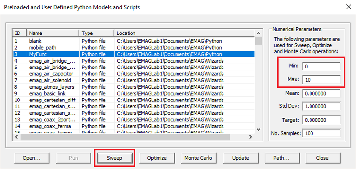
For single-variable Python functions, EM.Cube's modes dialog provides an easy way of performing a sweep, optimization of Monte Carlo simulation. Three buttons labeled Sweep, Optimize and Monte Carlo are intended for this purpose. In the case of sweep, you must enter Min and Max values for the sweep variable as well as Number of Samples. Select and highlight the name of your Python function from the list and click the Sweep button to run the sweep. At the completion of the sweep, the sweep data are saved in the file "MyFunc_sweep.DAT". Click the Data Manager ![]() button of Simulate Toolbar, or use the keyboard shortcut Ctrl+D, or select the menu item Simulate → Data Manager. Select the file "MyFunc_sweep.DAT" from the list by clicking on its name and highlighting its row in the table. Click the Plot button of the dialog. A graph of your sweep data is plotted in PyPlot.
button of Simulate Toolbar, or use the keyboard shortcut Ctrl+D, or select the menu item Simulate → Data Manager. Select the file "MyFunc_sweep.DAT" from the list by clicking on its name and highlighting its row in the table. Click the Plot button of the dialog. A graph of your sweep data is plotted in PyPlot.
In the case of optimization, you must enter Min and Max values for the optimization variable as well as a Target value for your Python function. Select and highlight the name of your Python function from the list and click the Optimize button to run the optimization. An objective function of the form e(x) = |func_name(x) - Target| is constructed and minimized. After the optimization algorithms converge, the optimal value of x and the optimization error are reported in the command window.
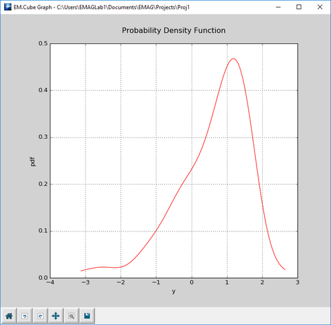
In the case of Monte Carlo simulation, you must enter values for Mean and Std Dev of the sweep variable as well as Number of Samples. Select and highlight the name of your Python function from the list and click the Monte Carlo button to run the simulation. Through this process, the probability density function (PDF) of your observable y = func_name(x) is estimated, and its graph is plotted as a function of y in PyPlot (file "MyFunc_mc.DAT" from the Data Base list). The mean and standard deviation of y are also reported in the command window.


