Difference between revisions of "EM.Picasso Tutorial Lesson 10: Optimizing A Microstrip Patch Antenna Design"
Kazem Sabet (Talk | contribs) |
Kazem Sabet (Talk | contribs) (→Setting Up the Optimization Process) |
||
| Line 136: | Line 136: | ||
</table> | </table> | ||
| − | Keep the default optimization '''Algorithm''' | + | Keep the default optimization '''Algorithm Type''', which is "Powell's Method". Next, you need to define the optimization variables. Similar to the case of a parametric sweep, on the left side of the dialog you will see a list of all the available independent variables already defined in your project. Select and highlight "recess_dep" and click the right arrow {{key|-->}} button in the middle of the dialog to move the selected variable to the '''Optimization Variables''' list on the right. A new dialog titled "Edit Optimization Variable" opens up. Enter 2 and 16 for the minimum and maximum values, respectively. Keep the default '''Variable Precision''' value of 0.1. Similarly, move "recess_wid" to the optimization variables table and enter 1 and 8 for its minimum and maximum values, respectively. |
<table> | <table> | ||
| Line 145: | Line 145: | ||
</table> | </table> | ||
| − | Back in the optimization settings dialog, you will see the specifications of the two optimization variables in the table on the right. | + | Back in the optimization settings dialog, you will see the specifications of the two optimization variables in the table on the right. Set the value of '''Maximum Error''' equal to 0.1. This is used for the convergence of the objective function or error function. You can see from the figure below that the error function or "goal" has been defined by the mathematical expression: |
| + | |||
| + | ---- | ||
| + | |||
| + | |20*log10(S11M) - (-20)| | ||
| + | |||
| + | ---- | ||
<table> | <table> | ||
Revision as of 15:06, 30 September 2016
Contents
What You Will Learn
In this tutorial you will revisit the rectangular patch antenna design with a recessed feed, which you explored earlier in Tutorial Lesson 2. This time, however, you will define a design objective and will use EM.Picasso's optimization utility to optimize the values of designated design variables to achieve your goal.
Getting Started
Open the EM.Cube application and switch to EM.Picasso. Start a new project with the following parameters:
Creating the Patch Geometry with a Recessed Feed
Follow a similar procedure as in Tutorial Lesson 2 and use the Microstrip-Fed Patch Wizard to create the parameterized geometry of a patch antenna with a recessed feed.
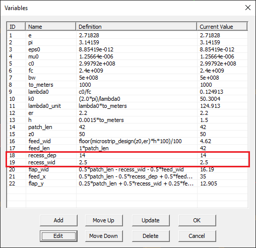
Open the variables dialog and make the following changes:
| Variable Name | Original Definition | New Definition |
|---|---|---|
| patch_len | floor(0.5*lambda0_unit*100/sqrt(er))/100 | 42 |
| recess_dep | 0.015*to_meters | 15 |
| recess_wid | 0.005*to_meters | 5 |
Defining the Design Objective
In this project, you will fix the side dimensions of the patch ("patch_len"), and will optimize the two feed variables: "recess_dep" and "recess_wid". But first you need to define a design objective for your project. The goal here is to achieve a good impedance match by varying the design variables. A return loss of -20dB typically represents a very good impedance match.
To define a design objective, click on the Objectives ![]() button of the Simulate Toolbar or select the menu item Simulate → Objectives... EM.Cube's Objectives dialog opens up, which is initially empty.
button of the Simulate Toolbar or select the menu item Simulate → Objectives... EM.Cube's Objectives dialog opens up, which is initially empty.
Click the Add button of this dialog to open "Add Objective" dialog. At the bottom of this dialog you will see a list of EM.Cube's available standard output parameters. The contents of this list varies depending on the observables you have already define for your project. Since the wizard created a port definition for this project, you will see a number of standard output parameters related to the S/Z/Y parameters. A design objective is defined as a logical statement:
expression_1 logical operator expression_2
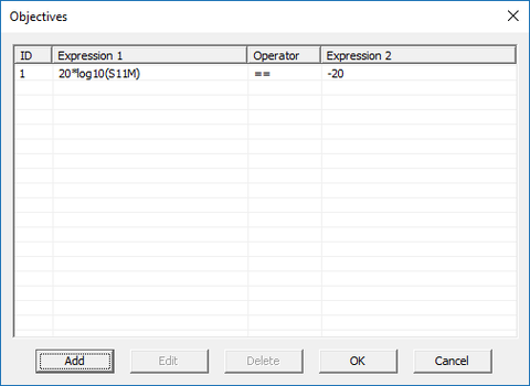
The first and second expressions can be any mathematical expression involving the standard output parameters, variables, Python functions, etc. The logical operators are "==", "<", "<=", ">", ">=" and "!=" (Not Equal To). If you set the mouse focus at one of the expression boxes and then double-click on the name of one of the output parameters in the list, it will be inserted in that box. Set up the following design objective as shown in the figure below:
20*log10(S11M) == -20
Close the "Add Objective" dialog to return to the Objectives dialog. You will see your new design objective added to the current objectives list. Close this dialog, too, and return to the project workspace.
Setting Up the Optimization Process
Open the simulation run dialog and select Optimization from the drop-down list labeled Simulation Mode.
Click the Settings button next to this drop-down list to open the Optimization Settings dialog.
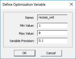
Keep the default optimization Algorithm Type, which is "Powell's Method". Next, you need to define the optimization variables. Similar to the case of a parametric sweep, on the left side of the dialog you will see a list of all the available independent variables already defined in your project. Select and highlight "recess_dep" and click the right arrow --> button in the middle of the dialog to move the selected variable to the Optimization Variables list on the right. A new dialog titled "Edit Optimization Variable" opens up. Enter 2 and 16 for the minimum and maximum values, respectively. Keep the default Variable Precision value of 0.1. Similarly, move "recess_wid" to the optimization variables table and enter 1 and 8 for its minimum and maximum values, respectively.
Back in the optimization settings dialog, you will see the specifications of the two optimization variables in the table on the right. Set the value of Maximum Error equal to 0.1. This is used for the convergence of the objective function or error function. You can see from the figure below that the error function or "goal" has been defined by the mathematical expression:
|20*log10(S11M) - (-20)|
Close the parametric sweep settings dialog and return to the run dialog. Click the Run key to start the parametric sweep. After the completion of the sweep simulation, open the data manager and plot the data file "S11_Sweep.CPX" in EM.Grid. Note that the return loss is minimized for the value recess_dep = 14mm.
Running a Parametric Sweep of the Feed Recess Width
Open the variable dialog and change the value of the variable "recess_dep" to 14mm.
Next, you are going to vary the width of the feed recess to see how far you can improve the return loss (|S11|). Open the simulation run dialog and then the parametric sweep settings dialog. Select and highlight "recess_dep" in the sweep variables table on the right side of the dialog. Click the left arrow <-- button in the middle of the dialog to move the selected sweep variable back to the Independent Variables list on the left. Now, select "recess_wid" from the left table and move it to the right table to make it the active sweep variable. In the "Edit Sweep Variable" dialog, accept the Uniform variable type and enter 1, 8, 1, for the start, stop and step values of the sweep variable, respectively. This will create a list of sweep variable values. Return to the parametric sweep settings dialog as shown in the figure below.
Run the new parametric sweep and then plot the data file "S11_Sweep.CPX" in EM.Grid. Note that the return loss is minimized for a value of recess_dep between 2mm and 3mm.
Analyzing the Patch Antenna with the Optimal Recessed Feed
You already set the value of the variable "recess_dep" to 14mm in the previous part. Now open the variables dialog again and change the value of the variable "recess_wid" to 2.5mm.
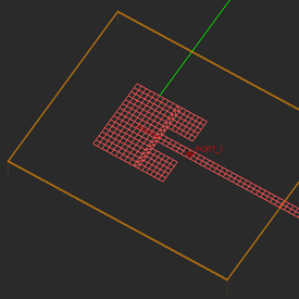
After the above changes, your patch antenna structure should look like this:
Run a quick single-frequency PMOM analysis of the optimal structure. At the end of the simulation, the port characteristics are reported as follows:
S11: 0.011933 +0.142894j
S11(dB): -16.869538
Z11: 49.134305 +14.336804j
Y11: 0.018756 -0.005473j
The return loss has dramatically improved down to -16.87dB. Visualize the current distribution and 3D radiation pattern of the antenna as shown in the figures below. Notice how the standing wave pattern has diminished on the microstrip feed line due to the improved impedance match.
Finally, run an adaptive frequency sweep of your patch antenna with the optimal recessed feed over the frequency range [2GHz, 3GHz]. After the completion of the sweep simulation, open the data manager and plot the data files "S11_RationalFit.CPX" and "Z11_RationalFit.CPX" in EM.Grid. The graphs of the S and Z parameters are shown in the figures below. A very good resonance and impedance match is accomplished at 2.4GHz.


