EM.Terrano Tutorial Lesson 9: Modeling A Mobile Communications Link Using Python

What You Will Learn

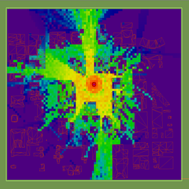
In this tutorial lesson, you will use EM.Cube's Python scripting capability. You will write Python functions to model a mobile path in the Downtown Ann Arbor propagation scene. Your Python functions will be used to define sweep variables associated with the coordinates of your transmitter's base location.

Back to EM.Terrano Manual

Back to EM.Terrano Tutorial Gateway

Download projects related to this tutorial lesson

Getting Started

Open the EM.Cube application and switch to EM.Terrano. If you downloaded the Ann Arbor template project in the previous tutorial lesson, open it again and save it as "EMTerrano_Lesson9". Otherwise, download the template project by clicking this link, and then open the downloaded project. Set the center frequency of the project to 5.8GHz. The table below summarizes the project parameters:

Use the Basic Link Wizard to create a vertically polarized dipole transmitter and a grid of isotropic receivers. Use the following parameters for the wizard:

Parameter Name	Default Value	New Value
area_size	250	450
Transmitter Height	10	2.5
Receiver Height	1.5	1.5
Receiver Spacing	5	5

The transmitter height of 2.5m corresponds to a vehicle-mounted antenna. Open the property dialog of the transmitter's base location point called "TXP" and change its X- and Y-coordinates to -90m and -150m, respectively. Your Ann Arbor scene should look like the figure the below:

The Ann Arbor scene propagation scene showing the transmitter location.

Writing a Python Script to Define the Mobile Path

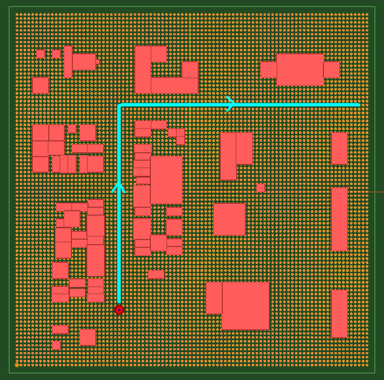
You want to move your transmitter around the city and see how the coverage map is affected due to the multipath effects. Since the height of the transmitter will stay fixed (vehicle-mounted), you will need two functions that determine the X and Y coordinates of the transmitter's base location, i.e. Point_1, at each step or instant of time. The Figure below shows the mobile path of the transmitter across the scene. It consists of two segments:

1. Vertical segment between (-90, -150, 2.5) and (-90, 110, 2.5) with 13 20m steps along the +Y axis
2. Horizontal segment between (-90, 110, 2.5) and (210, 110, 2.5) with 15 20m steps along the +X axis

The mobile path of the transmitter across downtown Ann Arbor.

You can write a Python function with an integer argument n representing the index of the successive points the transmitter traverses along the path. There are a total of 29 points starting from n = 0 and ending at n = 28. Two Python functions are indeed needed, one for the X-coordinate and the other for the Y-coordinate of the transmitter's based location as the variable n varies over its range. You are going to call these functions "mobile_path_x(n)" and "mobile_path_y(n)", respectively.

You can write a Python script in any text editor outside EM.Cube. But EM.Cube also provides a convenient utility for creating and managing Python functions. For this purpose, click the Models button of the Simulate Toolbar or select the menu item Simulate → Python Models & Scripts... to open the Models Dialog.

EM.Cube's models dialog.

This dialog provides a comprehensive list of all the preloaded python functions and scripts as well as your own user-defined Python functions. Select any file from the list and click the Open button of the dialog to open it in a text editor of your choice, which you have associated with the ".PY" file extension in Microsoft Windows. Two common choices are Windows Notepad or Notepad++.

EM.Cube also provides a blank Python file called "blank.PY" that is located in the folder "Documents → EMG → Python" and can be used as a template for your scripts. Select "blank.PY" from the list and open it. First, save the file as "mobile_path.PY" to change its name. The portion of the function that you have to enter in the provided template is given below:

def mobile_path_x(n):
	#Write your python code here
	if n<=13:
		return -90.0
	else:
		return -90.0 + (n-13)*20.0

def mobile_path_y(n):
	#Write your python code here
	if n<13:
		return -150.0 + n*20.0
	else:
		return 110.0

In Python, consistent indentation is very important. You can indent code lines either using the tab key or using a certain number of spaces, but you cannot mix both ways in the same script.

The figure below shows the entire script in Notepad++.

The Python file "mobile_path.PY" opened in the text editor Notepad++.

Once your Python script is complete, you can load it to EM.Cube using the Update button of the Models dialog and use it at the command line. Sometimes you might have to exit the EM.Cube application and open it again to use your new Python function.

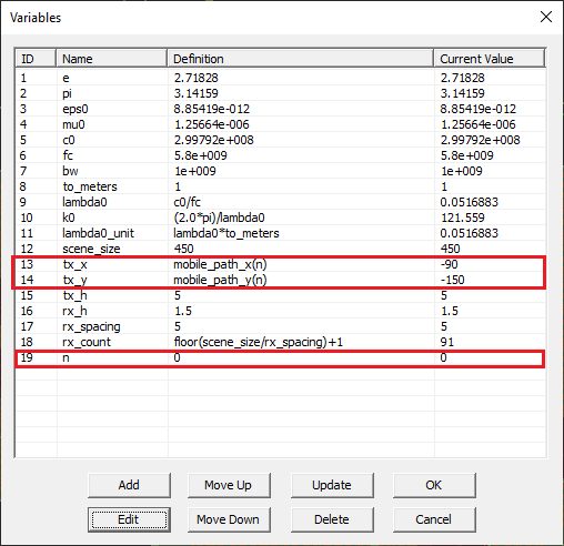
Now, open the variable dialog and define a new variable n = 0. Next, open the property dialog of the point object "Point_1" and replace the numeric values of its X and Y coordinates as follows:

Parameter Name	Original Value	New Value
X-coordinate	-90	mobile_path_x(n)
Y-coordinate	-150	mobile_path_y(n)

Initiating the index variable "n" in the variables dialog.

Changing the LCS coordinates of the transmitter's base location to Python functions.

Testing a Dry Run of Your Mobile Propagation Scene

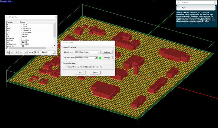
You can give different values to your variable "n" and verify the location of the transmitter. It is often useful to try a dry run of your variables before committing to a real sweep simulation. Open EM.Terrano's simulation run dialog and select Parametric Sweep as the simulation mode. Open the parametric sweep settings dialog, designate "n" as the sweep variable and set its start, stop and step values to 0, 28 and 1, respectively.

Defining the sweep variable "n".

The parametric sweep settings dialog showing "n" as the sweep variable.

While still in the parametric sweep settings dialog, click the Dry Run button of this dialog. You will see that the transmitter starts moving in the project workspace. In other words, the sweep variable n step through all of its designated samples and your physical structure gets updated for each sample. This results in an animation of the physical structure in the project workspace. A dry run is a safe way to test the extreme values of your variables before starting a time consuming sweep simulation. The dry run dialog works similar to animation controls dialog. You can change the speed of the dry run from this dialog.

The dry run dialog.

Running a Parametric Sweep Simulation of Your Mobile Propagation Scene

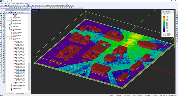
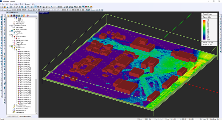
You are now ready to run a parametric sweep simulation of your project. Start the sweep and wait until all the 29 individual SBR simulations are completed. Then, visualize the coverage map and animate it.

The receive power coverage map of the Ann Arbor scene corresponding to the first position of the mobile transmitter.

The receive power coverage map of the Ann Arbor scene corresponding to the 9th position of the mobile transmitter.

The receive power coverage map of the Ann Arbor scene corresponding to the 14th position of the mobile transmitter.

The receive power coverage map of the Ann Arbor scene corresponding to the 21st position of the mobile transmitter.

The receive power coverage map of the Ann Arbor scene corresponding to the last (29th) position of the mobile transmitter.

Animating Your Coverage Maps

You can animate the coverage map plots in the project workspace. Right-click on the name of the receiver set "RX1" in the navigation tree and select Animation from the contextual menu. The 29 coverage maps start to appear in the project workspace consecutively and in an infinite loop. The Animation Controls dialog pops up at the lower right corner of the screen. From this dialog you can modify the animation frame rate in milliseconds. Use the Esc key to stop the animation.

VIDEO: Animation of top view of the coverage map of the Ann Arbor scene corresponding to the last position of the mobile transmitter.

---

Back to the Top of the Page

Back to EM.Terrano Tutorial Gateway