EM.Terrano Tutorial Lesson 7: Parametric Study Of A Realistic Urban Scene
Contents
What You Will Learn
In this tutorial, first you will import the CAD models of buildings in downtown Ann Arbor, MI. Then, you will learn how to perform a uniform frequency sweep and a parametric sweep of your propagation scene with the sweep variable being the transmitter height. You will also examine the statistical features of your SBR simulations.
![]() Back to EM.Terrano Tutorial Gateway
Back to EM.Terrano Tutorial Gateway
![]() Download projects related to this tutorial lesson
Download projects related to this tutorial lesson
Getting Started
Open the EM.Cube application and switch to EM.Terrano. Start a new project with the following parameters:
For this tutorial lesson, you need to download the STL model file containing the CAD models of the buildings. The file is called "AnnArborDowntown.STL" and features a simplified model of part of the University of Michigan's Central Campus in downtown Ann Arbor, MI. To download the file click here.
Constructing the Downtown Ann Arbor Scene
For this tutorial lesson, you will create a large terrain profile in the project workspace. Right-click on the Penetrable Surfaces item in the Physical Structure section of the navigation tree and select Insert New Terrain… from the contextual menu. The terrain surface group "Terrain_1" you created remains active for drawing new objects. Draw a rectangle, by clicking the Rectangle Strip ![]() button of the Object Toolbar or select the menu item Object → Surface → Rectangle Strip.
button of the Object Toolbar or select the menu item Object → Surface → Rectangle Strip.
Please note that external CAD objects are always imported to CubeCAD ![]() first. From CubeCAD you can transfer all or some of the imported object to any of the other computational modules. For this lesson, first create an impenetrable surface group called Block_1 in EM.Terrano's navigation tree with all the default settings. This means that your buildings will have the default dark brown color and their material composition would be "Brick" with εr = 4.4 and σ = 0.001S/m. Check the box labeled Adjust Blocks to Terrain Elevation to place building objects on the surface of the terrain.
first. From CubeCAD you can transfer all or some of the imported object to any of the other computational modules. For this lesson, first create an impenetrable surface group called Block_1 in EM.Terrano's navigation tree with all the default settings. This means that your buildings will have the default dark brown color and their material composition would be "Brick" with εr = 4.4 and σ = 0.001S/m. Check the box labeled Adjust Blocks to Terrain Elevation to place building objects on the surface of the terrain.
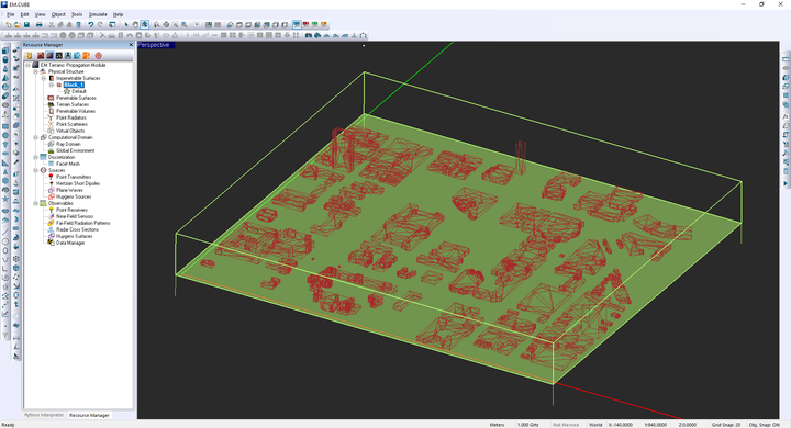
To import the building models, go to the File Menu and select Import.... The standard Windows Open Dialog opens up with the file type set to .STL. Browse your folders to find the downloaded "AnnArborDowntown.STL" file. An object appears in the project workspace of the CubeCAD Module as shown in the figure below.
Next, you have to move all the imported buildings to the Block_1 group of the EM.Terrano. To do so, select the building names on the navigation tree: Default. Right-click on the selection and select Move To → EM.Terrano → Block_1 from the contextual menu. All the objects will disappear from CubeCAD and will reappear in EM.Terrano's navigation tree under the "Block_1" group. If the imported building model contains many solid objects, e.g., Solid_1, Solid_2, …. Solid_n, in order to move all the imported buildings to the Block_1 group of the EM.Terrano, select all the building names on the navigation tree. Start with Solid_1 and select it. Then hold down the keyboard's Shift key and click Solid_n. While still holding down the shift key, right-click on the selection and select Move To → EM.Terrano → Block_1 from the contextual menu.
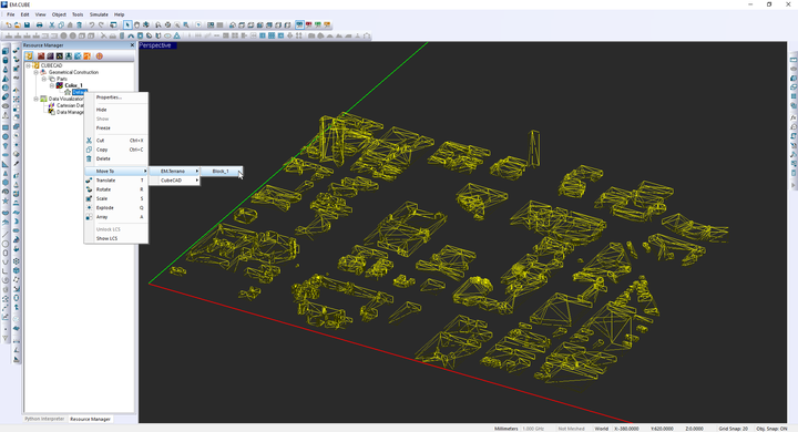 Moving the imported impenetrable building models from CubeCAD to the Block_1 group of the EM.Terrano. |
Defining the Transmitter & Receivers
Use the Basic Link Wizard to create a vertically polarized dipole transmitter and a grid of vertically polarized dipole receivers. Use the following parameters for the wizard:
| Parameter Name | Default Value | New Value |
|---|---|---|
| area_size | 500 | 850 |
| Tx Location X | 0 | 425 |
| Tx Location Y | 0 | 425 |
| Transmitter Height | 10 | 5 |
| Receiver Height | 1.5 | 1.5 |
| Receiver Spacing | 5 | 10 |
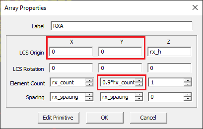
The point radiators corresponding to the receivers called "RXA" is originally positioned at (0.5*scene_size, 0.5*scene_size, tx_h) = (-425m, -425m, 1.5m). Change its coordinates to (0, 0, tx_h) and change the Element Count along the Y direction to 0.9* rx_count. This creates a very dense grid of 86×77 receivers.
Running a Uniform Frequency Sweep Simulation of the Urban Scene
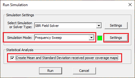
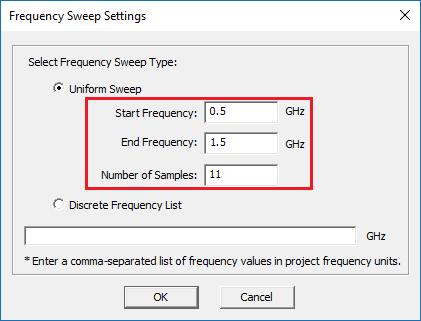
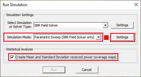
In the first part of this tutorial lesson, you will perform a frequency sweep simulation of your propagation scene. Open EM.Terrano's Simulation Run dialog and select Frequency Sweep as the simulation mode. Click on the Settings button next to this drop-down list to open the Frequency Sweep Settings dialog. In the frequency sweep settings dialog, select Uniform Sweep as the sweep type and set the values of the start and stop frequency to 0.5GHz and 1.5GHz, respectively, and set the number of frequency samples to 11. This will result in a frequency step of 100MHz. In the simulation run dialog, also check the box labeled Create Mean and Standard Deviation received power coverage maps in the "statistical Analysis" section of the dialog.
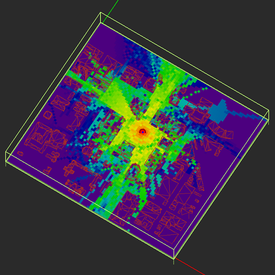
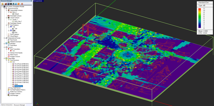
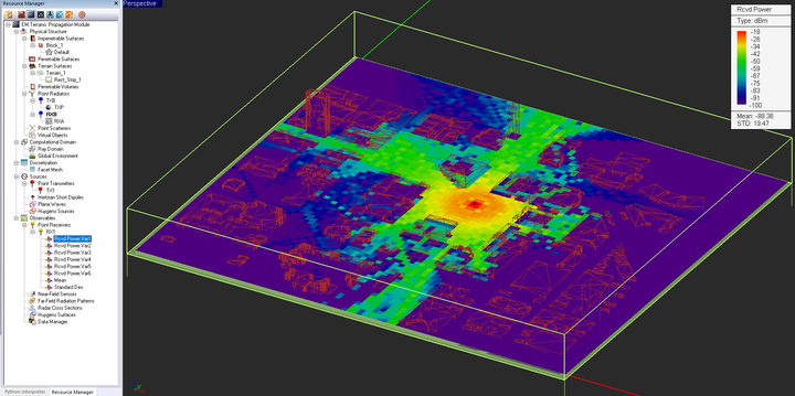
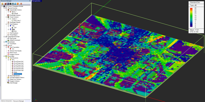
Now start the frequency sweep simulation of the Ann Arbor scene. At the end of the sweep simulation, a total pf 13 coverage maps are generated in the Observables sections of the navigation tree under the Point Receivers set node. Of these, the first 11 maps correspond to the received power at each of the 11 frequency samples from 500MHz to 1.5GHz. The last two plots are the mean and standard deviation coverage maps over the specified frequency range.
Performing a Parametric Sweep of Transmitter Height
In a parametric sweep simulation, one or more variables or parameters are varied, and the simulation engine is run for each parameter set. Open the Simulation Run dialog and choose the Parametric Sweep option from the Simulation Mode drop-down list. Click on the Settings button next to this drop-down list to open the Sweep Settings dialog.
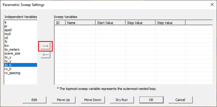
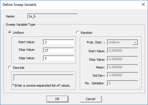
The sweep variables list is initially empty. On the left side of this dialog, you see a list of all the available independent variables. Select the transmitter height variable "tx_h" from the left table and used the --> button to move it to the right table. Another dialog titled "Sweep Variable" opens up. You have to set the start, stop and step values of your sweep variable. By default, the sweep variable is of uniform type. Enter 2, 27, and 5 for start, stop and step values, respectively. This will create a value list of {2, 7, 12, 17, 22, 27}. Close the sweep variable dialog and then close the sweep settings dialog to return to the simulation run dialog. Uncheck the box labeled Create Mean and Standard Deviation received power coverage maps in the run dialog.
Run the sweep simulation. At the end of the parametric sweep, a total of eight coverage maps appear in the Observables section of the navigation tree, one for each transmitter height value and the last two representing the mean and standard deviation maps.
