EM.Terrano Tutorial Lesson 3: Analyzing A Multipath Outdoor Propagation Scene

What You Will Learn

In this tutorial you will define impenetrable and penetrable surface blocks to model your building objects. You will learn how to define material properties of buildings and how to create CAD objects of different geometrical shapes to represent buildings. You will also investigate EM.Terrano’s facet mesh generator.

Back to EM.Terrano Manual

Back to EM.Terrano Tutorial Gateway

Download projects related to this tutorial lesson

Getting Started

Open the EM.Cube application. In the New Project Dialog, enter "EMTerrano_Lesson3" as the title of your new project. From the drop-down list labeled Problem Type, select "Simple Outdoor Propagation Scene - EM.Terrano". Keep the default choices of project’s Length Units, Frequency Units, Center Frequency and Bandwidth. Click the Create button of the dialog to return to the project workspace. A propagation scene is automatically created the contains two buildings, a transmitter and a grid of receivers.

Choosing the outdoor propagation scene template from the New Project dialog.

Start a new project with the following attributes:

Examining the Outdoor Scene Template

The template automatically creates a new block group called "BUILDING" under the Impenetrable Surfaces node in the Physical Structure section of the navigation tree. There are two box objects called "Building_1" and "Building_2" under the "BUILDING" group. Material or object groups are used in the navigation tree to group all the geometric objects with the same material and other physical properties as well as the same color and texture. For example, impenetrable surface blocks are used to represent and group impenetrable buildings. The faces of impenetrable buildings reflect the incident rays, and their edges diffracts the rays. However, rays cannot penetrate inside such buildings. This is a simple model for fast outdoor SBR analysis, when you are not concerned with multipath propagation inside the buildings. You can assume that impenetrable buildings have highly absorptive interiors such the the transmitted rays cannot leave the other side of the building and cannot return to the free space.

Geometric objects with different geometric shapes can belong to the same block group. All the objects belonging to a block group share the same color, texture and material properties.

The outdoor propagation scene template created by the New Project dialog.

Select the item "BUILDING" in the navigation tree. Right-click on it and select Properties... from the contextual menu. This opens up the Impenetrable Surface dialog, where you can see the color and material properties of this impenetrable surface group. In this case, the relative permittivity of the walls is ε_r = 4.44 and σ = 0.001S/m, which are typical of brick. You can change the material properties using the Add/Edit button. You can also build multilayer walls by adding new material layers to the stack.

EM.Terrano's Impenetrable Surface dialog.

The two buildings are box objects, the simplest and most widely used solid objects in EM.Cube. To open the property dialog of an object, either double-click on its surface, or right-click on its surface and select Properties... from the contextual menu. You can also do the same using the contextual menu of the two box items in the navigation tree. From the property dialog, you can see that the length, width and height of the two box objects have been parameterized. You can modify the values of the project variables from the Variable Dialog.

The property dialog of the box object.

The template created a blue point object called "Point_TX1" under the point radiators group "Base_TX1" as well as an orange point array called "Array_RX1" under the point radiators group "Base_RX1". A default vertically polarized half-wave dipole transmitter called "TX1" and an isotropic receiver grid called "RX1" were also created associated with "Base_TX1" and "Base_RX1", respectively. All of these were done automatically by the New Project dialog. Also note that a large number of receivers fall inside the two buildings. If a transmitter falls inside an impenetrable building, its rays will not reach any receivers outside the building. Similarly, if a receiver is located inside an impenetrable building, it will not receive any rays, and therefore, it will have a zero total received power.

If you hover your mouse over the surface of an object, its faces become translucent, and you see its inside.

Seeing through objects and viewing their interior using mouse-over.

Running an SBR Simulation of Your Outdoor Propagation Scene

Run a single-frequency SBR simulation of your scene and visualize its received power coverage map.

The perspective view of the received power coverage map of the receiver set.

You can clearly see the shadow regions behind the two buildings. From the navigation tree, enable the ray visualization. Open the property dialog of the receiver set and set the active receiver to receiver No. 167.

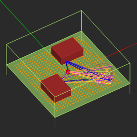
Visualizing the rays received by the receiver.

The ray data dialog of receiver No. 167 is shown in the figure below. A total of ten rays are received by this receiver.

Viewing the properties of individual rays in the ray data dialog.

You can sort the entries of the ray data dialog based on its parameters. For example, it is often useful to sort the rays based on their delay. To do so, simply click on the header of the delay columns in the table. As you would expect, the ray with the shortest delay time is the direct (LOS) ray.

Sorting the received rays based on their delay in ascending order.

Next, open the data manager and plot the following data files: "SBR_RX1_DELAY.DAT", "SBR_RX1_PhiARRIVAL.DAT", "SBR_RX1_ThetaARRIVAL.DAT", "SBR_RX1_PhiDEPARTURE.DAT", and "SBR_RX1_ThetaDEPARTURE.DAT" one by one.

Since EM.Cube graphs are interactive, you can open only one plot window at a time.

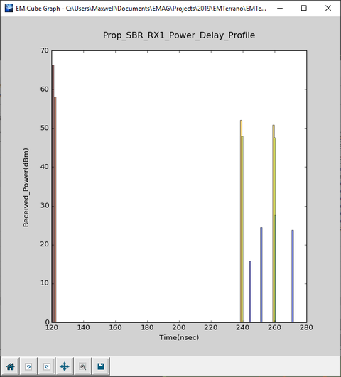The power delay bar chart graph for receiver No. 167.

The polar chart graph of Phi angles of arrival for receiver No. 167.	The polar chart graph of Theta angles of arrival for receiver No. 167.
The polar chart graph of Phi angles of departure for receiver No. 167.	The polar chart graph of Theta angles of departure for receiver No. 167.

Adding a New Penetrable Surface Block Group

Unlike impenetrable buildings, rays can penetrate buildings and objects that belong to a penetrable surface block group. Surface objects that belong to a such a block group act as thin walls that transmit he incident rays. Solid objects belonging to a penetrable surface block group are assumed to be hollow, and their faces represent thin walls.

To define a penetrable surface group, right-click on the Penetrable Surfaces item in the Physical Structure section of the navigation tree and select Insert New Block… from the contextual menu. This opens up the Penetrable Surface dialog with a default label "Block_2". The default color is light brown and the default material is “Brick”. Also note that the Wall Thickness is 0.5m for all the objects belonging to this block group.

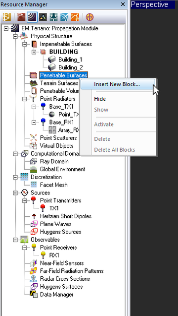Defining a penetrable surface group in EM.Terrano.

EM.Terrano's default Penetrable Surface dialog.

EM.Terrano's Edit Layer dialog.

EM.Cube's mateirals list.

All the objects belonging to the same penetrable surface group have the same wall thickness.

To change the material properties of the walls, select the current item in the table and click the Add/Edit button of the dialog. A new Edit Layer dialog opens up, showing the material properties of brick. Click the Material button to open up EM.Cube's Materials Dialog. You want to create a stone building. Typing "S" on your keyboard will take you down the table where the material names start with the letter S. Select "Stone" from the table and click OK to return to the Edit Layer dialog. You will see the new stone properties fill all the fields. Change the value of Wall Thickness to 0.2m. Close this dialog to return to the Penetrable Surface dialog.

EM.Terrano's Edit Layer dialog.

You will see the new material properties, ε_r = 2.12 and σ = 0.139S/m, for stone in the property table.

Changing the material properties in the Penetrable Surface dialog.

Drawing a New Penetrable Building with a Curved Geometry

The penetrable surface group "Block_2" you created in the last section remains active for drawing new objects. In this section, you are going to draw the geometry of a silo consisting of a cylindrical base and a hemispherical dome. Click the Cylinder button of the Object Toolbar or select the menu item Object → Solid → Cylinder.

Selecting the Cylinder Tool from the Object Toolbar.

With the cylinder tool selected, click on a blank space in the project workspace and drag the mouse to draw the circular base of your cylinder object. Your new building should have a radius of 15m. A property dialog pops up on the lower right corner of your screen. As you drag the mouse, you will see the base radius value continuously change. When the base reaches a size of 15m or something close to that, click the mouse. Next, you have to give the right height to your cylinder. Drag the mouse upward until you reach a height (Z-dimension) of 20m. Then, drop the mouse. You will see a light brown cylinder in the project workspace with a number of red edit handles on its base and top. Next, you have to move the new cylinder to the location. Set the LCS center of the cylinder to the point (40m, -40m, 0).

The Cylinder object's property dialog.

As you hover the mouse over the surface of the cylinder, you can snap to its characteristic point such as the center of its top face as shown in the figure below.

Snapping the mouse to the center of the top face of the cylinder object.

Next, click the Sphere button of the Object Toolbar or select the menu item Object → Solid → Sphere.

Selecting the Sphere Tool from the Object Toolbar.

With the sphere tool selected, snap to the center of the top face of the cylinder object and drag the mouse to draw the circular cross section of your sphere object. The radius of of sphere should be 15m, too. You can snap to the cylinder's side snap point to drop the mouse to set the LCS center of the sphere to the point (40m, -40m, 20). Note that your new object is a full sphere by default. In order to turn it to a hemisphere, you must set its End Angle to 180°.

The Sphere object's property dialog.

The four brick buildings on the global ground.

The table below summarizes the properties of the two objects you drew to model a silo:

Object	Geometry	Block Group	Surface Type	Material	Radius	Height	Location Coordinates	Start Angle	End Angle
Cylinder_1	Cylinder	Block_2	Penetrable surface	Stone	15m	20m	(40, -40m, 0)	0°	360°
Sphere_1	Sphere	Block_2	Penetrable surface	Stone	15m	N/A	(40m, -40m, 20m)	0°	180°

Discretizing the Scene Using the Mesh Generator

EM.Terrano uses a triangular surface mesh generator to discretize all the objects in the project workspace. This discretization is needed because the EM.Terrano's SBR simulation engine uses a locally flat representation of surfaces for the calculation of reflection and transmission coefficients. To view the triangular surface mesh of your buildings, click the Show/Generate Mesh button of the Simulate Toolbar or alternatively use the keyboard shortcut Ctrl+M. Note how the cylindrical object has been discretized into a number of flat triangular facets. In general, the mesh view shows how the simulation engine sees your physical structure. In the mesh view mode, you can perform view operations such as rotate view, zoom in/out or pan view, but you cannot select objects or edit them. To exit the mesh view mode and return to the normal view mode, use the keyboard’s Esc key or click the Show/Generate Mesh button of the Simulate Toolbar one more time.

The default triangular surface (facet) mesh of the building objects.

The facet mesh generator discretizes objects based on a Cell Edge Length parameter. This length is expressed in the project units and determines the approximate size of the triangular cells’ three sides. Its default value is 100 project units, which is a very large number. This default value works well as long as all the buildings of your scene are cubic, i.e. box objects. Since all the six faces of a box object are flat rectangles, they are discretized as four diagonal triangles. But at this coarse resolution, you might not produce a good representation of curved surfaces. EM.Terrano's facet mesh generator first tessellates objects with some raw triangles and then regularizes the mesh to produce triangular cells of almost equal size. To mesh curved surfaces, besides the cell edge length parameter, you can also change tessellation parameters.

You can set the mesh parameters by clicking the Mesh Settings button of the Simulate Toolbar or using the keyboard shortcut Ctrl+G or via the menu item Simulate → Discretization → Mesh Settings to open the SBR Mesh Settings Dialog.

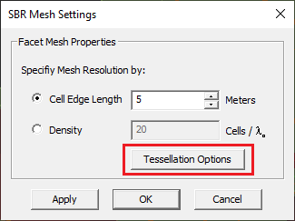EM.Terrano's Mesh Settings dialog.

Increase the mesh resolution by setting the value of the cell edge length equal to 5m. Then, click the Tessellation Options button and change the value of Curved Edge Angle Tolerance to 15° in the Tessellation Options Dialog. Close the latter dialog to return to the Mesh Settings dialog.

EM.Terrano's Mesh Settings dialog.

Click the Apply button to regenerate the fact mesh. This time you will get a more accurate reproduction of your buildings.

The high-resolution facet mesh of the building objects.

Running an SBR Analysis of the New Scene with Silo

At this time, run a quick SBR analysis of your propagation scene and visualize the received power coverage map. A lot of times, the buildings may obscure the view of a coverage map, or you may have receivers inside penetrable buildings that are concealed. You can hide any object or freeze it. In the freeze state, you will only see a wireframe outline of the object. To freeze an individual object, right-click on its surface in the project workspace or right-click on its name in the navigation tree and select Freeze from the contextual menu. To unfreeze an object, repeat the same procedure. You can also freeze all the objects belonging to a particular material or block group. In that case, you need to freeze the entire group using its contextual menu.

Freezing an individual object in EM.Terrano.

The received power coverage map of the new multipath scene with all the buildings in freeze state.

From the above coverage map, you can see that that the receivers located inside the silo receive a good amount of power. Next, visualize the rays in your propagation scene. The figure below show the rays collected by receivers No. 140 and No. 145. In the latter case, you see a very large number of rays that result from internal reflections from the walls of the penetrable building.

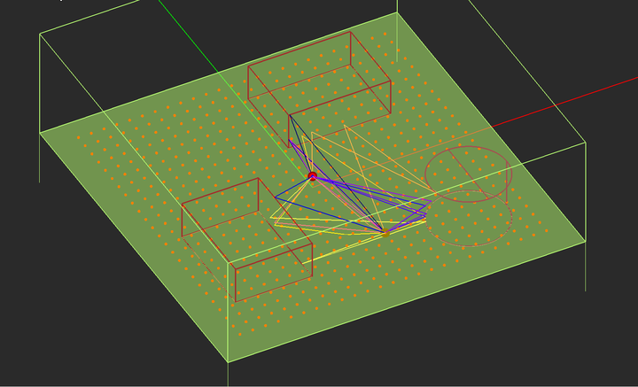Ray visualization for receiver No. 140 in the open area.

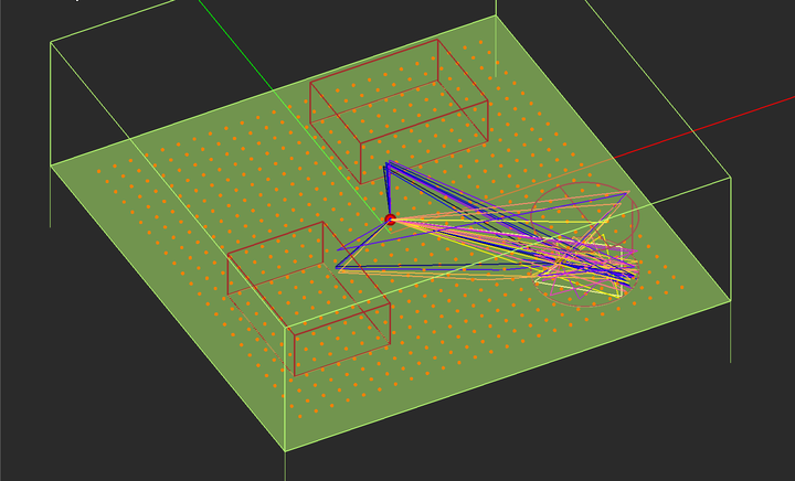Ray visualization for receiver No. 145 inside the silo.

---

Back to the Top of the Page

Back to EM.Terrano Tutorial Gateway