EM.Tempo Tutorial Lesson 7: Designing A Pyramidal Horn Antenna
Contents
What You Will Learn
In this tutorial you will build pyramidal horn antennas with different geometrical properties and aspect ratios and will analyze their radiation properties. You will also learn to use EM.Cube's Python command line and will write you own Python scripts to perform some mathematical calculations.
![]() Back to EM.Tempo Tutorial Gateway
Back to EM.Tempo Tutorial Gateway
![]() Download projects related to this tutorial lesson
Download projects related to this tutorial lesson
Getting Started
Open the EM.Cube application and switch to EM.Tempo. Start a new project with the following attributes:
Building the Pyramidal Horn Geometry
Click on the Horn Antenna Wizard ![]() button of the Wizard Toolbar or select the menu item Tools → Antenna Wizards → Pyramidal Horn Antenna.
button of the Wizard Toolbar or select the menu item Tools → Antenna Wizards → Pyramidal Horn Antenna.
The geometry of a pyramidal horn antenna with a rectangular waveguide feed appears in the project workspace. You are going to change the waveguide dimensions to those of a standard WR-650 waveguide. Open the variables dialog and make the following changes:
| Variable Name | Original Definition | New Definition |
|---|---|---|
| wg_a | waveguide_design(1.0,fc)*1.1*to_meters | 16.51 |
| wg_l | 0.5*lambda0_unit | 20 |
| wg_off | 0.25*lambda0_unit | 10 |
The wizard already defined a waveguide port source in the middle of the waveguide feed as well as two orthogonal near-field sensor planes and a far-field radiation pattern observable.
Running an FDTD Simulation of the Horn Antenna
Before running an FDTD analysis of your structure, let's take a close look at its mesh. Generate and view the mesh of the horn antenna with the default mesh density of 20 cells per wavelength. Since your project's center frequency is 1.2GHz with a bandwidth of 0.6GHz, the highest frequency of the project is 1.5GHz with a free-space wavelength of 20cm. Once the mesh appears on the screen, pay attention to EM.Tempo’s Status Bar. Next to the units and frequency sections of the status bar, you will see a number triplet: 183 × 150 × 113, in this case. These are the numbers of FDTD mesh grid lines inside the computational domain along the X, Y and Z directions, respectively. If you subtract each number by one, you will get the number of mesh cells in each direction. It is important to keep in mind that besides the visible computational domain in the project workspace, the FDTD simulation engine also sees a number of PML layers behind the domain walls. By default, there are six 8-layer CMPL walls embracing your computational domain. Therefore, your FDTD project involves a total of (183 -1 + 2×8) × (150 -1 + 2×8) × (113 -1 + 2×8) = 197 × 164 × 127 = 4,181,760 mesh cells.
| |
When simulating very large computational problems, EM.Tempo's GPU-accelerated FDTD engine can speed up the solution significantly if your computer has a powerful GPU card with enough onboard RAM memory. |
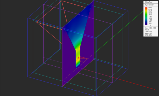
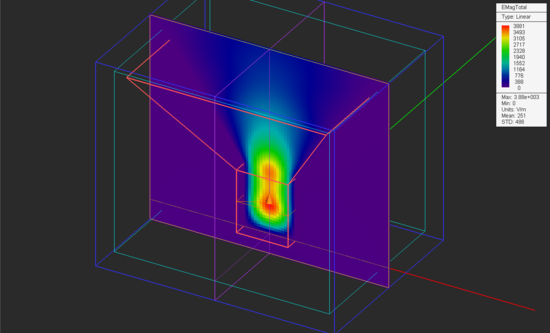
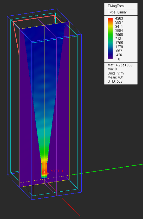
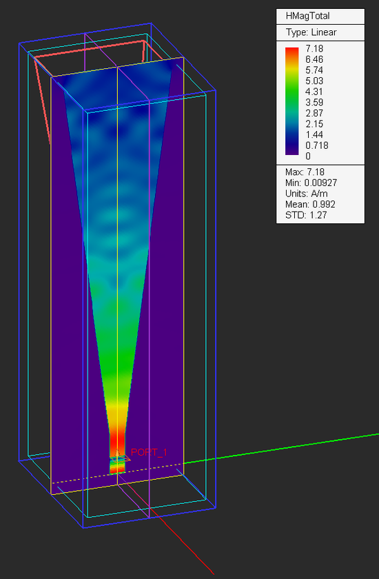
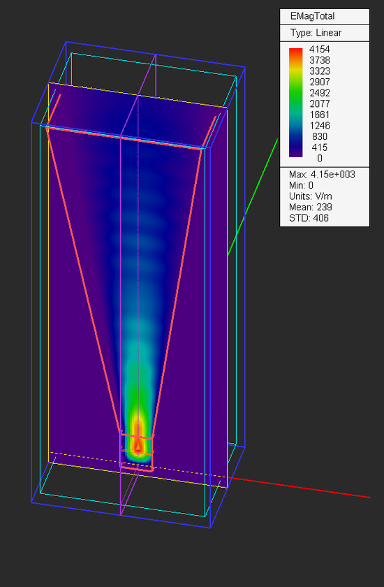
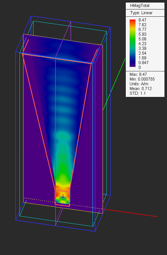
Run an FDTD Analysis of your horn antenna structure and examine the electric and magnetic field distributions on the two sensor planes.
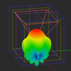
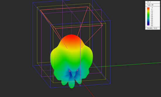
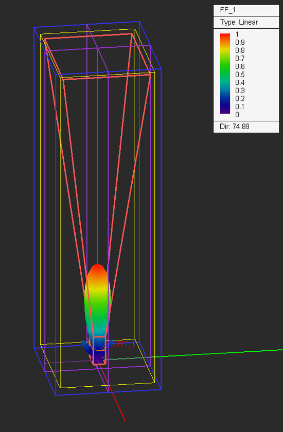
Visualize the 3D radiation pattern of the waveguide-fed horn antenna in both linear and dB scales.
From the variables dialog you can see that the value of the variable "gain_dB" was set to 15dB. Also, the aperture dimensions and length of the pyramidal horn section were chosen based on design formulas to yield an antenna gain of 15dB. From the 3D radiation pattern plot, you can see that the computed directivity of your horn structure is 15.02dB.
Designing a Long Horn Antenna
In this section of the tutorial lesson, you are going to change the aperture dimensions and length of the pyramidal horn section according to the table below:
| Variable Name | Original Definition | New Definition |
|---|---|---|
| horn_aperture_a | horn_design_a(gain_dB,wg_a/lambda0_unit,wg_b/lambda0_unit)*lambda0_unit | 80 |
| horn_aperture_b | horn_design_b(gain_dB,wg_a/lambda0_unit,wg_b/lambda0_unit)*lambda0_unit | 60 |
| horn_len | horn_design_l(gain_dB,wg_a/lambda0_unit,wg_b/lambda0_unit)*lambda0_unit | 200 |
Your horn antenna geometry should now look like this:
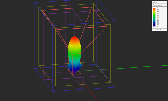
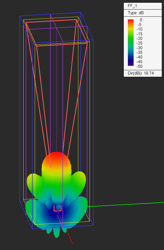
After meshing the longer horn, you will see a new number triplet in the status bar: 231 × 185 × 279. The total number of mesh cells can be calculated as (231 -1 + 2×8) × (185 -1 + 2×8) × (279 -1 + 2×8) = 245 × 199 × 295 = 14,464,800 mesh cells. This is a fairly large computational problem. Run an FDTD analysis of the new horn structure and plots its near-field distributions and far-field radiation patterns.
From the radiation pattern plots, you can see that the directivity of the longer horn has increased to 18.74dB.
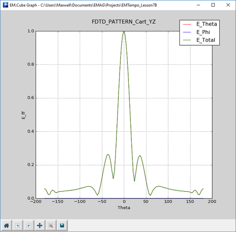
The figures below show the 2D Cartesian and polar graphs of the radiation patterns in the principal E-plane and H-plane of the horn antenna.
Verifying Your Simulation Results
In order to verify your simulation results, you will consider the approximate analytical expressions for the directivity of a pyramidal horn antenna of aperture dimensions A × B and length L fed by a rectangular waveguide of dimensions a × b. These are given by:
[math] D_P = \frac{4\pi AB}{\lambda_0^2} \epsilon_t \epsilon_E \epsilon_H [/math]
where
[math] \epsilon_t = \frac{8}{\pi^2} [/math]
[math] \epsilon_H = \frac{\pi^2}{64t} \left[ \left[ C(p_1) - C(p_2) \right]^2 + \left[ S(p_1) - S(p_2) \right]^2 \right] [/math]
[math] \epsilon_E = \frac{\left[ C(q) \right]^2 + \left[ S(q) \right]^2}{q^2} [/math]
[math] t = \frac{1}{8R_{0H}/\lambda_0} \left( \frac{a}{\lambda_0} \right)^2 [/math]
[math] p_1 = 2\sqrt{t} \left( 1+ \frac{1}{8t} \right) [/math]
[math] p_2 = 2\sqrt{t} \left( -1+ \frac{1}{8t} \right) [/math]
[math] q = \frac{b}{\sqrt{2\lambda_0 R_{0E}}} [/math]
and the pyramidal radii R0H and R0E are given by:
[math] R_{0H} = \frac{L}{1-a/A} [/math]
[math] R_{0E} = \frac{L}{1-b/B} [/math]
For your pyramidal horn antenna, A = 80cm, B = 60cm, L = 200cm, a = 16.51cm, b = 8.255cm and λ0 = 25cm. Therefore, the pyramidal radii are R0H = 252.008cm and R0E = 231.906cm, and t = 0.005408.
In the above formulas, C(x) and S(x) are the Fresnel cosine and sine integral functions. These are advanced mathematical functions expressed as complicated integrals that can only be evaluated numerically. EM.Cube provides a large set of advanced mathematical function as Python libraries or modules. For example, you can find the syntax of the Fresnel integral functions from EM.Cube's functions list. To open this list, click the Functions ![]() button of the Simulate Toolbar or select the menu item Simulate → Functions....
button of the Simulate Toolbar or select the menu item Simulate → Functions....
Python is a versatile scripting language that can be used very effectively for all kinds of mathematical calculations. You can use EM.Cube's Python Command Line as an online calculator or execute sophisticated Python scripts. The figure below shows some of the above calculations using Python's command line:
Based on the above calculations, you will find that p1 = 3.546579, p2 = 3.252418 and q = 0.076661. The approximate analytical value of the directivity of the pyramidal horn antenna is finally found as:
[math] \epsilon_t = 0.8106, \quad \epsilon_H = 0.999979, \quad \epsilon_E = 0.999992 [/math]
[math] D_p= \frac{(4\pi)(0.8)(0.6)}{(0.25)^2} (0.8106)(0.999979)(0.999992 ) = 78.226 = 18.93dB[/math]
which agrees fairly well with the directivity value computed by EM.Tempo.
Writing a Python Script for Calculation of Pyramidal Horn Directivity
At the last step of this tutorial lesson, you will write your own first Python function to calculate the directivity of a pyramidal horn antenna. The input and output of such a function are:
INPUTS: l0 (m), a (m), b (m), A (m), B (m), L (m)
OUTPUT: D0
You can write a Python script in any text editor outside EM.Cube. But EM.Cube also provides a convenient utility for creating and managing Python functions. For this purpose, click the Models ![]() button of the Simulate Toolbar or select the menu item Simulate → Python Models & Scripts... to open the Models Dialog.
button of the Simulate Toolbar or select the menu item Simulate → Python Models & Scripts... to open the Models Dialog.
This dialog provides a comprehensive list of all the preloaded python functions and scripts as well as your own user-defined Python functions. Select any file from the list and click the Open button of the dialog to open it in a text editor of your choice, which you have associated with the ".PY" file extension in Microsoft Windows. Two common choices are Windows Notepad or Notepad++.
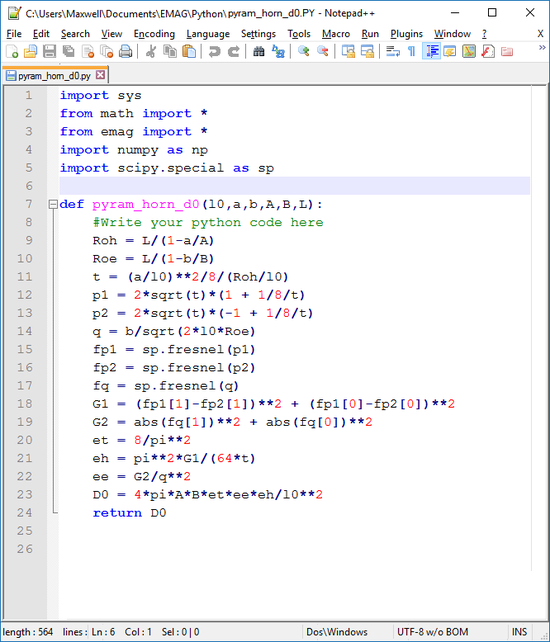
EM.Cube also provides a blank Python file called "blank.PY" that is located in the folder "Documents → EMG → Python" and can be used as a template for your scripts. Select "blank.PY" from the list and open it. First, save the file as "pyram_horn_d0.PY" to change its name. The portion of the function that you have to enter in the provided template is given below:
def pyram_horn_d0(l0,a,b,A,B,L):
#Write your python code here
Roh = L/(1-a/A)
Roe = L/(1-b/B)
t = (a/l0)**2/8/(Roh/l0)
p1 = 2*sqrt(t)*(1 + 1/8/t)
p2 = 2*sqrt(t)*(-1 + 1/8/t)
q = b/sqrt(2*l0*Roe)
fp1 = sp.fresnel(p1)
fp2 = sp.fresnel(p2)
fq = sp.fresnel(q)
G1 = (fp1[1]-fp2[1])**2 + (fp1[0]-fp2[0])**2
G2 = abs(fq[1])**2 + abs(fq[0])**2 et = 8/pi**2
eh = pi**2*G1/(64*t)
ee = G2/q**2
D0 = 4*pi*A*B*et*ee*eh/l0**2
return D0
| |
In Python indentation is very important. You can indent using the tab key or using a certain number of spaces, but you cannot mix the two ways in the same script. |
The figure below shows the entire script in Notepad++.
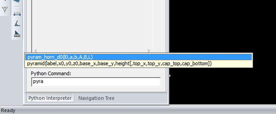
Once your Python script is complete, you can load it to EM.Cube using the Update button of the Models dialog and use it at the command line. If you start typing the name of your new Python function in the command line, a small tip window will appear that helps you remember the syntax of the command.
| |
Oftentimes you might have to exit the EM.Cube application and open it again to use your new Python functions. |
If you select the syntax and double-click on the tip window, it will be copied into the command window. Now you can replace the arguments with their numeric values relevant to this project:
l0 = 25m, a = 0.1651m, b = 0.08255m, A = 0.8m, B = 0.6m and L = 2m
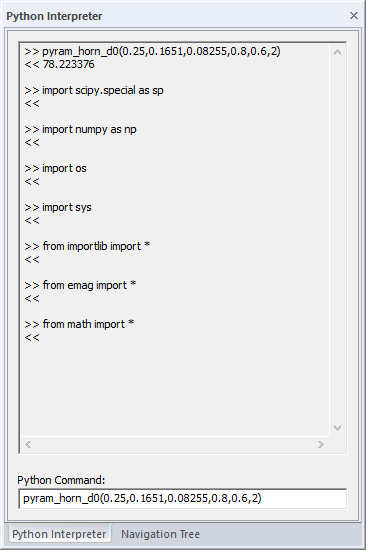
So, in the command line enter "pyram_horn_d0(0.25,0.1651,0.08255,0.8,0.6,2)" and hit the Enter key of the keyboard. The Python function is evaluated, and the result (D0 = 78.22) is reported on the screen.
