Advanced Tutorial Lesson 14: Fourier Analysis of Discrete-Time Sampled Signals
Contents
What You Will Learn
In this tutorial you will learn how to use RF.Spice's discrete-time Fourier transform (DTFT) blocks as well as its discrete Fourier transform (DFT) blocks. You will also learn how to define arbitrary temporal waveforms.
A Note on RF.Spice's Fourier Transform Blocks
RF.Spice A/D provides a number of virtual blocks for performing discrete-time Fourier transform operations. A discrete-time Fourier transform (DTFT) is applied to a discrete-time signal, which can be constructed from the samples of a continuous signal. Let's define the Fourier transform of a continuous signal x(t) of the time variable t in the following form:
[math] X(f) = \mathcal{F}\left \{ x(t)\right\} = \int_{-\infty}^\infty x(t)e^{-j 2 \pi f t} dt [/math]
together with its inverse transform:
[math] x(t) = \mathcal{F}^{-1}\left \{X(f)\right\} = \int_{-\infty}^\infty X(f)e^{j 2 \pi f t} df [/math]
If you sample the continuous signal x(t) with a sampling period of T, its samples can be represented by a discrete-time sequence in the integer variable n:
[math] x[n] = x(nT), \quad\quad n \in Z [/math]
The discrete-time Fourier transform (DTFT) of the sequence x[n] is then defined by:
[math] X_{1/T}(f) = T \sum_{n=-\infty}^{\infty} x[n] \ e^{-j 2\pi n f T} [/math]
Using the Poisson sum formula, we can relate the discrete-time Fourier transform X1/T(f) of the sequence of x[n] with the Fourier transform X(f) of the continuous-time signal x(t):
[math] X_{1/T}(f) = \sum_{k=-\infty}^{\infty} X\left(f - k/T\right) [/math]
The above equation means that the DTFT of x[n] is indeed a periodic version of X(f) in the frequency domain with a period of fs = 1/T.
Another interpretation of the DTFT is the Fourier transform of the impulse train made up of the samples of x(t):
[math] X_{1/T}(f) = \mathcal{F}\left \{\sum_{n=-\infty}^{\infty} x[n] \delta(t-nT)\right \} [/math]
where δ(t) is the Dirac delta function.
The Discrete Fourier Transform (DFT) of the discrete-time signal or sequence x[n] is defined by:
[math]X[k] = \sum_{n=0}^{N-1} x[n] e^{-j2 \pi k n / N} \quad k = 0, 1, 2, ..., N-1[/math]
which is an N-periodic sequence. The inverse discrete Fourier transform is given by:
[math] x[n] = \frac{1}{N} \sum_{k=0}^{N-1} X[k] e^{j 2 \pi k n / N} \quad n = 0, 1, 2, ..., N-1[/math]
RF.Spice A/D provides ten DTFT blocks and ten DFT blocks with different numbers of samples ranging from 5 to 64. These blocks all have a sampling period parameter T in seconds. The DFT blocks also have another parameter N which is the sequence length or the number of discrete-time samples. The default value of T = 1s means that the 5-point DTFT block operates on a total signal duration of 5s, while the 32-point DTFT block operates on a total signal duration of 32s. By the same token, the 32-point DTFT block with a sampling period of T = 250ms operates on a total signal duration of 32 × 0.25s = 8s.
The Fourier transform of a real-valued signal is typically a complex-valued function of the frequency. The DTFT can be written as:
[math] X_{1/T}(f) = \sum_{n=-\infty}^{\infty} x[n] \ \left[ \cos(2\pi n f T) - j \sin(2\pi n f T) \right] = X^c_{1/T}(f) -jX^s_{1/T}(f) [/math]
where the cosine and sine DTFT transforms are defined by:
[math] X^c_{1/T}(f) = \sum_{n=-\infty}^{\infty} x[n]\cos(2\pi n f T) [/math]
[math] X^s_{1/T}(f) = \sum_{n=-\infty}^{\infty} x[n]\sin(2\pi n f T) [/math]
Similarly, the DFT can be written as:
[math] X[k] = \sum_{n=0}^{N-1} x[n] \ \left[ \cos(2\pi kn/N) - j \sin(2\pi kn/N) \right] = X^c[k] -jX^s[k] \quad k = 0, 1, 2, ..., N-1 [/math]
where the cosine and sine DFT transforms are defined by:
[math] X^c[k] = \sum_{n=0}^{N-1} x[n]\cos(2\pi kn/N) [/math]
[math] X^s[k] = \sum_{n=0}^{N-1} x[n]\sin(2\pi kn/N) [/math]
All of RF.Spice's ten DTFT blocks and ten DFT blocks take a continuous signal as their input, sample it with a sampling period T specified by you, and produce two output signals corresponding to the cosine and sine DTFT or DFT transforms. It is very important for you to understand that the two output signals of the DTFT blocks are still constructed and plotted as functions of time. They are indeed time domain voltage signals that are computed through a transient simulation of your input signal, but they must be interpreted in the frequency domain by reinterpreting the time axis as a frequency axis (f ≥ 0). As a result, you can always see and plot only the positive frequency axis.
Computing the DTFT of a Pulse Waveform
The following is a list of parts needed for this part of the tutorial lesson:
| Part Name | Part Type | Part Value |
|---|---|---|
| V1 | Voltage Source | Waveform TBD |
| R1 | Resistor | 100 |
| X1 | 8-Point Discrete Time Fourier Transform Block | Defaults, T = 1s |
| X2 | Complex Modulus Block | Defaults |
Place and connect the parts as shown in the figure below. The Complex Modulus Block is used to output the absolute value or magnitude of the complex-valued spectral signal.
To generate a single pulse waveform of duration 8s, use the following parameters for the voltage source V1:
| Initial Voltage | 0 |
|---|---|
| Peak Voltage | 1 |
| Delay Time | 0 |
| Rise Time | 1ns |
| Fall Time | 1ns |
| Pulse Width | 8s |
| Pulse Period | 1e+20s |
Run a Transient Test of this circuit with the parameters specified below:
| Start Time | 0 |
|---|---|
| Stop Time | 20 |
| Linearize Step | 1ms |
| Step Ceiling | 1ms |
| Preset Graph Plots | v(1), v(2), v(3), v(4) |
The simulation results are shown in the figure below. As you would have expected, the output is a periodic sinc function.
The input signal (the yellow pulse in the above figure) can be expressed as:
[math] x(t) = rect \left( \frac{t-4}{8} \right) [/math]
whose complex Fourier transform is:
[math] X(f) = 8 \left[ \frac{\sin(8\pi f)}{8\pi f} \right] e^{-j8\pi f} [/math]
The figure below shows a zoomed-in version of the above figure over the time interval [10s, 12s] so you can better see the details of the waveforms. The period of the output period sinc function is fs = 1/T = 1/(1s) = 1Hz. Here you will interpret the horizontal axis as the frequency f-axis for the signals v(2), v(3) and v(4). Since the DTFT block samples the input signal every one second, you could have also input a pulse train of period 1s with 8 pulses instead. The outputs would have been identical. Note that in each period, the sinc function has 8 peaks.
Before moving to the next part, change the sampling period of the DTFT block to T = 0.5s and run another Transient Test of your circuit using the same parameters as before. Note that the 8-point DTFT block X1 will collect a total of 8 samples of your input signal v(1) at half-second intervals. This means that the DTFT block will see your input pulse waveform only over the time interval [0, 4s]. In other words, your input signal has been effectively reduced to:
[math] x_1(t) = rect \left( \frac{t-2}{4} \right) [/math]
whose complex Fourier transform is:
[math] X_1(f) = 4 \left[ \frac{\sin(4\pi f)}{4\pi f} \right] e^{-j4\pi f} [/math]
The figure below shows the new simulation results. Note that whereas the sampling period T has shrunk by half, the period of the output sinc signal has increased to fs = 1/T = 1/(0.5s) = 2Hz. This is expected from the scaling property of the Fourier transform. Note that the sinc function still has 8 peaks in each period.
Defining an Arbitrary Temporal Waveform
The following is a list of parts needed for this part of the tutorial lesson:
| Part Name | Part Type | Part Value |
|---|---|---|
| V1 | Arbitrary Temporal Waveform Generator | Waveform TBD |
| R1 | Resistor | 100 |
| X1 | 16-Point Discrete Time Fourier Transform Block | Defaults, T = 0.5s |
| X2 | Complex Modulus Block | Defaults |
Using RF.Spice's arbitrary temporal waveform generator, you can define any mathematical function of time as the waveform of your voltage source. You can access this generalized source from Menu > Parts > Waveform Generation Blocks > Basic Waveforms > Arbitrary Temporal Waveform Generator. In the property dialog of this source, click the Edit Model... button to open a second dialog where you need to enter a mathematical expression as a function of "v(t)". In other words, v(t) stands for the time variable.
In this part of the tutorial lesson, you will define a sinc function:
[math] x_2(t) = sinc(t) = \frac{\sin(\pi t)}{\pi t} [/math]
whose Fourier transforms is known to be:
[math] X_2(f) = rect(f) [/math]
For this purpose, you need to enter the following expression in the arbitrary source's property dialog:
sin( pi * v(t)) / ( pi * v(t))
Place and connect the part as shown in the figure below. This time you are using a 16-point DTFT block with a sampling period of T = 0.5s. This will provide an 8s window to the sinc function.
Run a Transient Test of this circuit with the parameters specified below:
| Start Time | 0 |
|---|---|
| Stop Time | 20 |
| Linearize Step | 1ms |
| Step Ceiling | 1ms |
| Preset Graph Plots | v(1), v(2), v(3), v(4) |
The simulation results are shown in the figure below. As you would have expected, the output is a periodic pulse function, or the periodic replicas of the "rect" function with a unit width and a period of 2Hz:
It is important to note that your finite-duration input signal as seen by the DTFT block's 8s time-limited window is indeed given by the following more sophisticated function:
[math] x_3(t) = sinc(t) . rect \left( \frac{t-4}{8} \right) [/math]
whose complex Fourier transform is given by the following frequency-domain convolution:
[math] X_3(f) = rect(f) * 8 \left[ \frac{\sin(8\pi f)}{8\pi f} \right] e^{-j8\pi f} [/math]
The above equation explains the fluctuations and aliasing effects you can clearly see in the above plots.
Next, replace the 16-point DTFT block with a 32-point DTFT block with the same sampling period of T = 0.5s:
This time you have enlarged the DTFT block's sampling window to 32 × 0.5s = 16s. Your input signal is now:
[math] x_4(t) = sinc(t) . rect \left( \frac{t-8}{16} \right) [/math]
whose complex Fourier transform is given by the following frequency-domain convolution:
[math] X_4(f) = rect(f) * 16 \left[ \frac{\sin(16\pi f)}{16\pi f} \right] e^{-j16\pi f} [/math]
Run another transient test of your new circuit with the same parameters as before. The results are shown in the figure below, which hasn't change much compare to the previous graph. The convolving frequency-domain sinc has been compressed more tightly. As a result, the reconstructed frequency-domain pulse output is cleaner and sharper.
Finally, set the sampling period of the 32-point DTFT block to T = 0.25s. This reduces the width of the DTFT block's sampling window back to 8s. Your input signal is now:
[math] x_5(t) = x_3(t) = sinc(t) . rect \left( \frac{t-4}{8} \right) [/math]
whose complex Fourier transform is given by the following frequency-domain convolution:
[math] X_5(f) = X_3(f) = rect(f) * 8 \left[ \frac{\sin(8\pi f)}{8\pi f} \right] e^{-j8\pi f} [/math]
Run one more transient test of your circuit with the same parameters as before. The results are shown in the figure below, where you can see a doubled spectral period of f<subs</sub> = 1/T = 1/(0.25s) = 4Hz, while the output pulse's unit width has remained the same as before.
Using Discrete Convolution Blocks
The following is a list of parts needed for this part of the tutorial lesson:
| Part Name | Part Type | Part Value |
|---|---|---|
| V1 | Finite Sequence Pulse Generator | Waveform TBD |
| R1 | Resistor | 100 |
| X1 | 16-Point Discrete Convolution Block | Defaults, T = 1s |
| 2 | 32-Point Discrete Convolution Block | Defaults, T = 0.5s |
| X3 | Discrete-Time Signal Hold Block | Defaults, T = 0.5s, Tmax = 20s |
The convolution of two continuous-time functions x(t) and h(t) is defined as:
[math] x(t) * h(t) = \int_{-\infty}^\infty x(\tau)\, h(t - \tau)\, d\tau [/math]
The convolution of two discrete-time signals x[n] and h[n] is defined as:
[math] f[n] * g[n] = \sum_{k=-\infty}^\infty x[k]\, h[n - k] [/math]
RF.Spice A/D provides ten Discrete Convolution blocks with different numbers of samples ranging from 5 to 64. You can access these block from Menu > Parts > Digital Signal Processing Blocks > Discrete Convolution Blocks. In this part of the tutorial lesson, you are going to convolve a pulse function with itself. For the input pulse you will use a Finite Sequence Pulse Generator which can be accessed from the same menu as the pulse (train) generator. To generate a pulse sequence of duration 8s, use the following parameters for the voltage source V1:
| pulse period (T) | 1s |
|---|---|
| pulse width (w) | 0.1s |
| Number of Pulses (n) | 9 |
| Rise Time | 1ms |
| Fall Time | 1ms |
| Maximum Output Voltage Level | 1V |
| Start Time | 0 |
From signal theory, we know that the output of the convolution is a triangular signal with a duration of 16s.
Place and connect the 16-point convolution block as shown in the figure below:
Run a Transient Test of this circuit with the parameters specified below:
| Start Time | 0 |
|---|---|
| Stop Time | 20s |
| Linearize Step | 1ms |
| Step Ceiling | 1ms |
| Preset Graph Plots | v(1), v(2) |
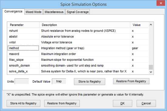
Before running the simulation, open RF.Spice's "SPICE Simulation Options" dialog and change the Integration Method from the default choice "trap" to "gear". Sometimes, the simulation may not converge quickly using the "trap" method.
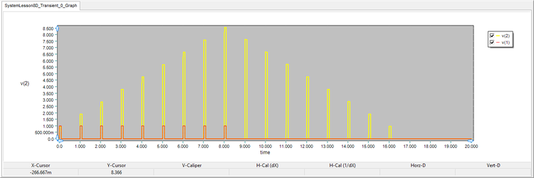
The simulation results are shown in the figure below, where you can see the resulting triangular function of double width.
Next, replace the 16-point convolution block with the 32-point convolution block, set its sampling period to T = 0.5s, and follow it with the Discrete-Time Signal Hold Block as shown in the figure below. Set the value of the sampling period T of this block equal to 0.5m and its Tmax parameter to 20s.
Change the parameters of the Finite Sequence Pulse Generator as follows:
| pulse period (T) | 0.5s |
|---|---|
| pulse width (w) | 0.05s |
| Number of Pulses (n) | 17 |
| Rise Time | 1ms |
| Fall Time | 1ms |
| Maximum Output Voltage Level | 1V |
| Start Time | 0 |
Run a Transient Test of this circuit with the parameters specified below:
| Start Time | 0 |
|---|---|
| Stop Time | 20s |
| Linearize Step | 0.5ms |
| Step Ceiling | 0.5ms |
| Preset Graph Plots | v(1), v(2), v(3) |
The simulation results are shown in the figure below. The total input signal duration is still 8s, but you have twice as many input samples this time.
Comparing & Contrasting DTFT and DFT Blocks
The following is a list of parts needed for this part of the tutorial lesson:
| Part Name | Part Type | Part Value |
|---|---|---|
| V1 | Finite Sequence Pulse Generator | T = 1s, w = 0.1s, N = 9, Rise Time = 1ms, Fall Time = 1ms |
| R1 -R2 | Resistor | 100 |
| X1 | 16-Point Discrete Convolution (DTCONV16) Block | Defaults, T = 1s, N = 32 |
| X2 | 16-Point Discrete Fourier Transform (DFT16) Block | Defaults, T = 1s |
| X3 | 16-Point Discrete-Time Fourier Transform (DTFT16) Block | Defaults, T = 1s |
| X4 - X5 | Complex Modulus Block | Defaults |
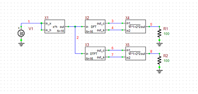
In this part of this tutorial lesson, you are going to take the discrete-time output signal of the convolution circuit of the previous part and pass it through DFT16 and DTFT16 blocks to calculate both the discrete-time Fourier transform (DTFT) and discrete Fourier transform (DFT) of the triangular pulse sequence. Set the Sequence Length of the DFT block to N = 48.
Place and connect all the parts as shown in the figure below:
Run a Transient Test of this circuit with the parameters specified below:
| Start Time | 0 |
|---|---|
| Stop Time | 20 |
| Linearize Step | 0.5ms |
| Step Ceiling | 0.5ms |
| Preset Graph Plots | v(2), v(3), v(4), v(5), v(6), v(7), v(8) |
For this simulation, too, change the SPICE integration method to "gear" in the SPICE Simulation Options dialog. The simulation results are shown in the figure below. You can see that the Fourier transform results stabilize after a quite long period of time.
The DFT results are indeed the samples of the DTFT results in the time interval [16s, 17s]. Zoom in the above graph and scale the time axis to the interval [15.5s, 17.5s] to better see the details. As you can see from the figures, your input signal is a triangular pulse sequence which is the result of convolution of a pulse sequence with itself. According to Parseval's theorem:
[math] \mathcal{F}\left \{ x(t) * h(t) \right \} = \mathcal{F}\left \{ x(t) \right \} \cdot \mathcal{F}\left \{ h(t) \right \} = X(f) \cdot H(f) [/math]
the Fourier transform of the convolution of the two "rect" functions must be a "squared sinc" function, which is clearly visible from the results.
The DFT samples are taken by default over one frequency period equal to 1/T. You can extend the sampling window to "n_dur / T" by setting a value greater than 1 for the n_dur parameter of the DFT block. Also, the frequency sampling starts by default at t = NDTFT.T + n_delay/T. The default value of the n_delay parameter of the DFT block is zero. It can take both positive or negative values.
Reconstructing the DFT of a Discrete-Time Sampled Signal
The following is a list of parts needed for this part of the tutorial lesson:
| Part Name | Part Type | Part Value |
|---|---|---|
| V1 | Finite Sequence Pulse Generator | T = 1s, w = 0.1s, N = 9, Rise Time = 1ms, Fall Time = 1ms |
| R1 -R2 | Resistor | 100 |
| X1 | 16-Point Discrete Convolution (DTCONV16) Block | Defaults, T = 1s |
| X2 | 16-Point Discrete Fourier Transform (DFT16) Block | Defaults, T = 1s, N = 64, Duty Cycle = 0.25 |
| X3 | Complex Modulus Block | Defaults |
| X4 | Discrete-Time Signal Hold Block | Defaults, T = 15.625ms, Tmax = 156.25ms |
Before closing this tutorial lesson, let's see what happens if you increase the DFT's sequence length or period N to 64. Place and connect the parts as shown in the figure below.
Open the property dialog of the DFT16 block called X2, set N = 64 and set the value of the sampling pulse Duty Cycle to 0.25. Since the sampling period is T = 1s, the spectral period is fs = 1Hz. With a sequence length of N = 64, the spectral contents will be sampled at fs/N = 1/(NT) = 1/64Hz = 15.625mHz. Remember that on the time axis this mean signal details on a time scale of 15.625ms. In other words, the DFT pulse sequence is located in the time interval [16s, 17s] with a pulse period of T′ = 15.625ms. This is the value that you will choose for the sampling period of the signal hold block. Set the value of the Tmax parameter of this block to 10T′ = 156.25ms.
Run a Transient Test of this circuit with the parameters specified below:
| Start Time | 0 |
|---|---|
| Stop Time | 20 |
| Linearize Step | 0.5ms |
| Step Ceiling | 0.5ms |
| Preset Graph Plots | v(5), v(6) |
The simulation results are shown in the figure below. Zoom in the graph's time axis and scale it to the interval [16s, 17s] to see the reconstructed spectral response.


