V&V Article 4: Designing Wideband Dielectric Resonator Antennas Using EM.Tempo

Introduction

In this verification & validation (V&V) article, we will analyze a number of wideband dielectric resonator antennas (DRA) using EM.Cube's FDTD Module, also known as EM.Tempo. Dielectric resonators are typically made of a block of high permittivity dielectric material on a metallic ground plane that is excited through some sort of feed mechanism. The material block acts as a dielectric resonator, and the antenna feed excites one or more characteristic modes of this resonator. In this article, we will investigate rectangular, spherical and cylindrical dielectric resonator antennas with different types of strip and slot feeds. Both linearly polarized (LP) and circularly polarized (CP) antenna designs will be considered.

Rectangular Dielectric Resonator Antennas

In the first part of this article, we consider a rectangular dielectric resonator antenna of dimensions a × b × h placed on a large metallic (PEC) ground plane as shown in Figure 1. The relative permittivity ε_r of the dielectric material must be high (typically 10 or larger), and its relative permeability is μ_r = 1.

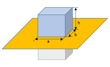Figure 1: Geometry of a dielectric resonator antenna consisting of a high permittivity dielectric block on a metallic ground plane. The figure also shows the image of the dielectric block in the PEC ground plane.

The modal characteristics equation of this dielectric resonator can be written as:

[math] k_x^2 + k_y^2 + k_z^2 = \left( \frac{m\pi}{a} \right)^2 + \left( \frac{n\pi}{b} \right)^2 + \left( \frac{l\pi}{h} \right)^2 = \epsilon_r k_0^2 [/math]

where k₀ = 2πλ₀ is the free space propagation constant and λ₀ is the free space wavelength. The integers m, n and l are the modal characteristic indices. The above equation assumes the effective height of the resonator to be 2h due to the image of the dielectric block in the PEC ground. The resonant frequency of the TEmnl mode is then found from the following equation:

[math] f_{res} = \frac{c}{2\pi\sqrt{\epsilon_r}} \sqrt{ \left( \frac{m\pi}{a} \right)^2 + \left( \frac{n\pi}{b} \right)^2 + \left( \frac{l\pi}{h} \right)^2 } [/math]

Rectangular DRA with an Edge Strip Feed

Figure 2 shows a rectangular dielectric resonator of dimensions 14.3mm × 25.4mm × 26.1mm and relative permittivity ε_r = 9.8, on a metallic ground plane of dimensions 60mm × 60mm, fed by a vertical metallic strip of width 1mm and height 9mm on one edge of the dielectric block. In practice, the strip is soldered to an SMA connector. For the purpose of electromagnetic simulation, the coaxial feed can be modeled by a lumped source placed between the lower edge of the strip and the ground plane.

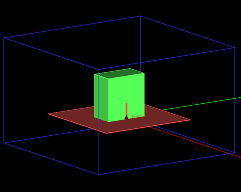Figure 2: Geometry of a dielectric resonator antenna with a vertical metallic strip on its edge fed by a coaxial line from underneath the ground plane.

According to the dielectric waveguide model (DWM) discussed in Ref. [2], this resonator configuration excites the following modes:

TE_z111: f_res = 3.95GHz

TE_z113: f_res = 4.7GHz

Figure 3 shows the return loss (|S₁₁|) of the dielectric resonator antenna simulated by EM.Tempo and compares it with the measured data given by Ref. [2]. It can be seen from this figure that EM.Tempo predicts these two resonant frequencies very well. A wide fractional bandwidth of abou 43% is observed. Figure 4 shows the real and imaginary parts of the input impedance of the antenna simulated by EM.Tempo and compares them with the measured data given by Ref. [2]. It must be noted that neither of the two references [1] or [2] give the exact dimensions of the ground plane.

Figure 3: Return loss of the dielectric resonator antenna of Figure 2, solid line: EM.Tempo results, and symbols: measured data given by Ref. [2].

Figure 4: Real and imaginary parts of the input impedance of the dielectric resonator antenna of Figure 2, solid red line: EM.Tempo results for input resistance, solid blue line: EM.Tempo results for input reactance, orange symbols: measured data given by Ref. [2] for input resistance, and turquoise symbols: measured data given by Ref. [2] for input reactance.

Figures 5 and 6 show the 2D polar radiation patterns of the DRA at f = 3.5GHz in the E-plane (ZX) and H-plane (YZ), respectively. Figures 7 and 8 show the 2D polar radiation patterns of the DRA at f = 4.3GHz in the E-plane (ZX) and H-plane (YZ), respectively. Figures 5-8 also compare EM.Tempo's simulated results with the simulation data presented by Ref. [1] and measured data given by Ref. [2]. The measured data are given for the upper half-space only, implying that a very large metallic ground plane might have been used to minimize the back radiation. The discrepancies between the two sets of simulated data might be due to the difference in the ground plane dimensions as the data in the upper half-space agree very well.

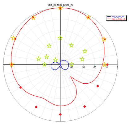Figure 9: E-plane (ZX) radiation pattern cut of the dielectric resonator antenna of Figure 2 at f = 3.5GHz, red solid line: EM.Tempo (FDTD) results for co-pol Eθ, red diamond symbols: simulated data presented by Ref. [1] for Eθ, orange star symbols: measured data presented by Ref. [2] for Eθ, blue solid line: EM.Tempo (FDTD) results for cross-pol Eφ, blue diamond symbols: simulated data presented by Ref. [1] for Eφ, and green star symbols: measured data presented by Ref. [2] for Eφ.

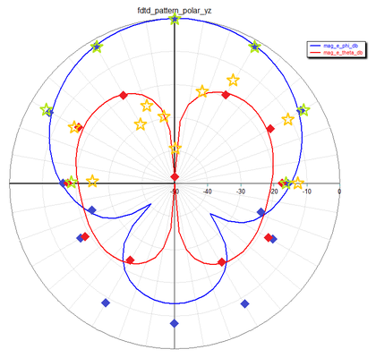Figure 6: H-plane (YZ) radiation pattern cut of the dielectric resonator antenna of Figure 2 at f = 3.5GHz, blue solid line: EM.Tempo (FDTD) results for co-pol Eφ, blue diamond symbols: simulated data presented by Ref. [1] for Eφ, green star symbols: measured data presented by Ref. [2] for Eφ, red solid line: EM.Tempo (FDTD) results for cross-pol Eθ, red diamond symbols: simulated data presented by Ref. [1] for Eθ, and orange star symbols: measured data presented by Ref. [2] for Eθ.

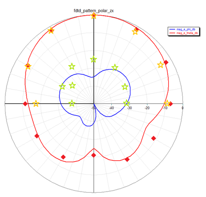Figure 7: E-plane (ZX) radiation pattern cut of the dielectric resonator antenna of Figure 2 at f = 4.3GHz, red solid line: EM.Tempo (FDTD) results for co-pol Eθ, red diamond symbols: simulated data presented by Ref. [1] for Eθ, orange star symbols: measured data presented by Ref. [2] for Eθ, blue solid line: EM.Tempo (FDTD) results for cross-pol Eφ, blue diamond symbols: simulated data presented by Ref. [1] for Eφ, and green star symbols: measured data presented by Ref. [2] for Eφ.

Figure 8: H-plane (YZ) radiation pattern cut of the dielectric resonator antenna of Figure 2 at f = 4.3GHz, blue solid line: EM.Tempo (FDTD) results for co-pol Eφ, blue diamond symbols: simulated data presented by Ref. [1] for Eφ, green star symbols: measured data presented by Ref. [2] for Eφ, red solid line: EM.Tempo (FDTD) results for cross-pol Eθ, red diamond symbols: simulated data presented by Ref. [1] for Eθ, and orange star symbols: measured data presented by Ref. [2] for Eθ.

Slot-Coupled Rectangular DRA

Next, we consider a slot-coupled dielectric resonator antenna. Figure 9 shows the geometry of the rectangular DRA with dimensions 10.5mm × 20.8mm × 18.5mm and relative permittivity ε_r = 10, on a metallic ground plane of dimensions 60mm × 75mm. Underneath the ground plane is a thin dielectric substrate of relative permittivity ε_r = 2.93 and thickness d = 0.762mm. The dielectric resonator is excited through a rectangular slot, which is fed by a microstrip line printed on the bottom side of the substrate. The microstrip line has a width of w_f = 1.94mm and extends beyond the coupling slot by a length Ls = 7.2mm. The slot is located at the center of the base of the resonator and its length and width are L = 10.6mm and w = 2.6mm, respectively. The microstrip line stretches all the way to the edge of the substrate, where it is excited by a microstrip port. According to the dielectric waveguide model (DWM) discussed in Ref. [3], this resonator configuration excites the following modes:

TE_z111: f_res = 3.47GHz

TE_z113: f_res = 5.30GHz

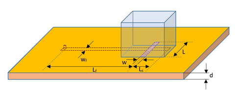Figure 9: Geometry of a slot-coupled dielectric resonator antenna with a microstrip feed line.

Figures 10 and 11 show screenshots of the EM.Tempo project depicting the slot-coupled rectangular dielectric resonator antenna.

Figure 10: Screenshot of the top side of the slot-coupled rectangular DRA in EM.Tempo showing the dielectric resonator at the top of the substrate.

Figure 11: The geometry setup for the slot-coupled rectangular DRA in EM.Tempo showing the coupling slot and the microstrip feed line on the bottom side of the substrate with some objects in freeze state.

This project was simulated using EM.Tempo, and the computed return loss of the DRA is plotted in Figure 12. This figure also shows the measured results presented by Ref. [3]. The measured values of the resonant frequencies are 3.4GHz and 5.18GHz for the two TE_z111 and TE_z113 modes, respectively. Similar to the previous case, the dimensions of the metallic ground planes were not given in Ref. [3].

Figure 12: Return loss of the dielectric resonator antenna of Figure 10, solid line: EM.Tempo results, symbols: measured data given by Ref. [3].

Figures 13 and 14 show the 3D far field radiation patterns of the DRA at the two resonant frequencies f = 3.4GHz and f = 5.2GHz. From these two figures, the directivity of the DRA is seen to be 6.84dBi and 8.04dBi at f = 3.4GHz and f = 5.2GHz, respectively. Ref. [3] reports measured antenna gain values of 4.02dBi at 3.48GHz and 7.52dBi at 5.13GHz. The lower gain values take into account the antenna losses that were not modeled by EM.Tempo. It should also be noted that the differences in the ground plane size might contribute to discrepancies in the computation of the antenna directivity.

Figure 13: 3D far field radiation pattern of the dielectric resonator antenna of Figure 10 computed at f = 3.4GHz by EM.Tempo.

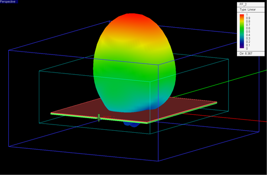Figure 14: 3D far field radiation pattern of the dielectric resonator antenna of Figure 10 computed at f = 5.2GHz by EM.Tempo.

Spherical DRA with a Conformal Strip Feed

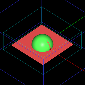
A spherical DRA is typically made of a hemispherical dielectric block placed on a metallic ground plane. Figure 15 shows the geometry of a spherical DRA of radius a = 12.5mm and relative permittivity ε_r = 9.5 with a conformal strip feed. The length of the conformal metal strip is 12mm and its width is 1.2mm. The conformal strip feed is modeled in EM.Tempo in a similar way as the strip feed of the rectangular DRA of Figure 2. A short wire containing a lumped source is used to connect the bottom end of the curved strip to the ground. The conformal strip can be readily created in EM.Cube using a vertically standing circle curve in the ZX principal plane with start and end angles of 5° and 55°, respectively, which corresponds to an arc of length 11mm. The circular curve is then converted to a strip using EM.Cube's "Strip Sweep" tool. The FDTD mesh of the spherical DRA is shown in Figure 16 with a mesh density of 30 cells/λ_eff. An adaptive mesh algorithm was used to adequately represent the curved surfaces of the hemispherical block and the conformal strip.

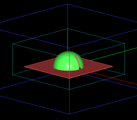Figure 15: Geometry of a spherical DRA with a conformal strip feed.

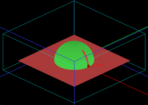Figure 16: FDTD mesh of the spherical DRA with a conformal strip feed.

Figure 17 shows the return loss (|S₁₁|) of the spherical dielectric resonator antenna simulated by EM.Cube's FDTD solver. Figure 18 shows the real and imaginary parts of the input impedance of the same antenna simulated by EM.Tempo and compares them with the simulated and measured data given by Ref. [5]. As in the previous examples, Ref. [5] does not give the dimensions of the metallic ground plane of the fabricated antenna. A PEC ground plane of dimensions 50mm × 50mm was used for the EM.Tempo simulation. Figure 19 shows the 3D far field radiation pattern of the spherical DRA at f = 2.5GHz.

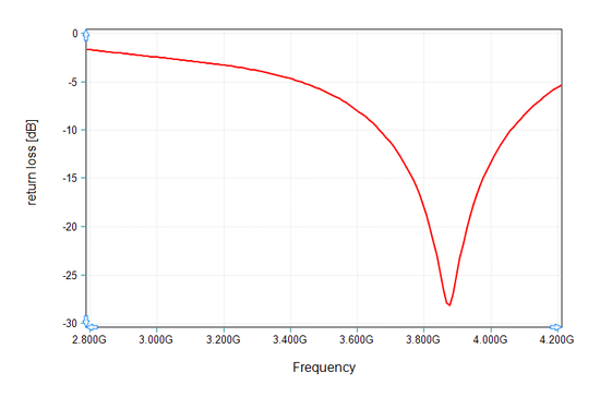Figure 17: Return loss of the spherical dielectric resonator antenna of Figure 15.

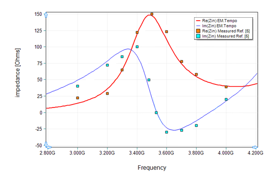Figure 18: Real and imaginary parts of the input impedance of the spherical dielectric resonator antenna of Figure 24, solid red line: EM.Tempo results for input resistance, solid blue line: EM.Tempo results for input reactance, orange symbols: measured data given by Ref. [5] for input resistance, and turquoise symbols: measured data given by Ref. [5] for input reactance.

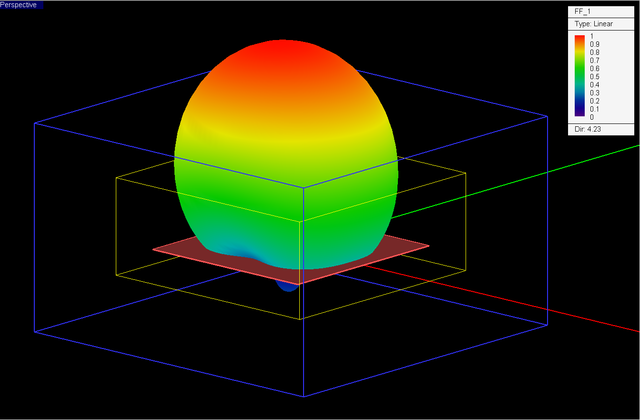Figure 19: 3D far field radiation pattern of the spherical dielectric resonator antenna of Figure 15 computed at f = 3.5GHz by EM.Tempo.

Slot-Coupled Spherical DRA

Just like a rectangular DRA, a spherical DRA can also be excited through a coupling slot. Figure 20 shows the geometry of a slot-coupled spherical DRA. The feed mechanism of this DRA is very similar to that of the rectangular DRA of Figure 10, consisting of a coupling slot in the metallic ground plane, which is fed by an underpassing microstrip line printed on a thin dielectric substrate on the other side of the ground plane. In Figure 20, the radius of the dielectric hemisphere is a = 12.5mm and its relative permittivity is ε_r = 9.5, which are identical to the case of Figure 15. The slot dimensions are L = 13.5mm and w = 0.9mm. The substrate has a thickness d = 0.635mm and a relative permittivity ε_r = 2.96. The microstrip feed line parameters are w_f = 1.45mm and L_s = 13.6mm. The feed line extends to the edge of the substrate, where it is excited using a microstrip port. The metallic ground dimensions are 100mm × 100mm.

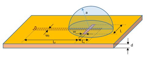Figure 20: Geometry of a slot-coupled spherical DRA with an underlying microstrip feed line.

Figures 21 and 22 show screenshots of the EM.Tempo project depicting the slot-coupled spherical dielectric resonator antenna.

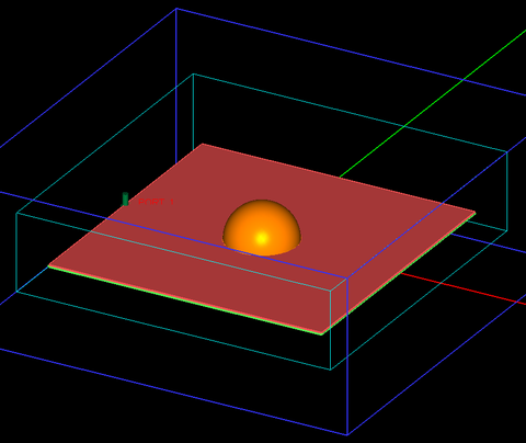Figure 21: Screenshot of the top side of the slot-coupled spherical DRA in EM.Tempo showing the dielectric resonator at the top of the substrate.

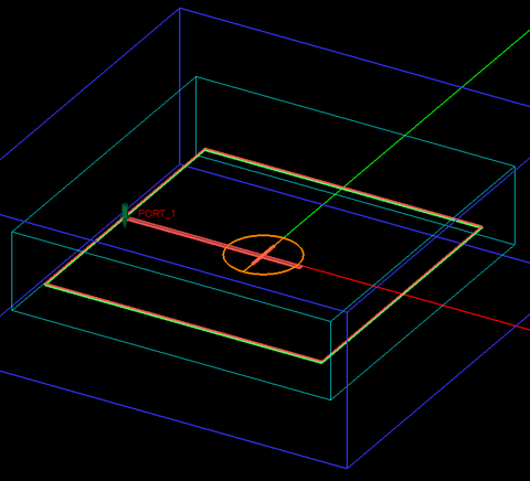Figure 22: The geometry setup for the slot-coupled spherical DRA in EM.Tempo showing the coupling slot and the microstrip feed line on the bottom side of the substrate with some objects in freeze state.

Figure 23 shows the return loss (|S₁₁|) of the slot-coupled spherical dielectric resonator antenna simulated by EM.Tempo. It also compares these results with the measured data presented by Ref. [6]. A very good agreement can be seen between the two sets of data. Figure 24 shows the 3D far field radiation pattern of the slot-coupled spherical DRA at f = 3.5GHz.

Figure 23: Return loss of the slot-coupled spherical dielectric resonator antenna of Figure 20, solid red line: EM.Tempo (FDTD) results, red symbols: measured data given by Ref. [6].

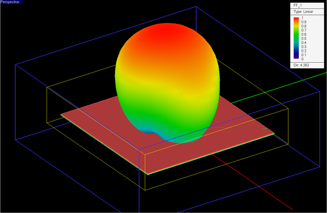Figure 24: 3D far field radiation pattern of the spherical dielectric resonator antenna of Figure 20 computed at f = 3.5GHz by EM.Tempo.

Coaxial Probe-Fed Spherical DRA

As the last example of spherical DRAs, we consider a spherical dielectric resonator with a coaxial probe feed as shown diagrammatically in Figure 25. The radius of the dielectric hemisphere is a = 12.5mm and its relative permittivity is ε_r = 9.8. The dielectric resonator is placed on a metallic ground plane of dimensions 60mm × 60mm and is fed by a coaxial transmission line of inner conductor radius r₁ = 0.63mm and outer conductor radius r₂ = 1.5mm. An air-filled coaxial line of these radii has a characteristics impedance of 50 Ohms. The coaxial cable is located underneath the ground plane and its outer conductor is grounded. The inner conductor of the coaxial probe is extended by a height of h = 6.5mm inside the dielectric block. The probe feed is offset from the center of the dielectric hemisphere by a length b = 6.4mm. To excite the coaxial probe in EM.Tempo, it is extended downward by a length L_f = 15mm. A coaxial port is placed at the bottom of the coaxial feed line. Figure 26 shows the construction of the physical structure in EM.Tempo, and Figure 27 shows the details of the coaxial feed.

Figure 25: The geometry of a spherical DRA with a coaxial probe feed.

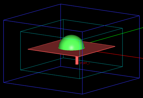Figure 26: Screenshot of a spherical DRA with a coaxial probe feed in EM.Tempo.

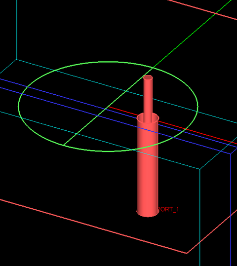Figure 27: Details of the coaxial feed of the spherical DRA of Figure 26 with most objects in their freeze state.

Figure 28 shows the computed return loss (|S11|) of the probe-fed spherical dielectric resonator antenna simulated by EM.Tempo. Figure 29 shows the real and imaginary parts of the input impedance of the same antenna simulated by EM.Tempo and compares them with the measured data given by Ref. [8]. According to the analysis presented in Ref. [8], this particular DRA excites the TM₁₀₁ and TE₂₂₁ modes with very close resonant frequencies of 5.245GHz and 5.267GHz, respectively. Figure 30 shows the 3D far field radiation pattern of this spherical DRA at f = 4.5GHz.

Figure 28: Return loss of the coaxial-fed dielectric resonator antenna of Figure 26.

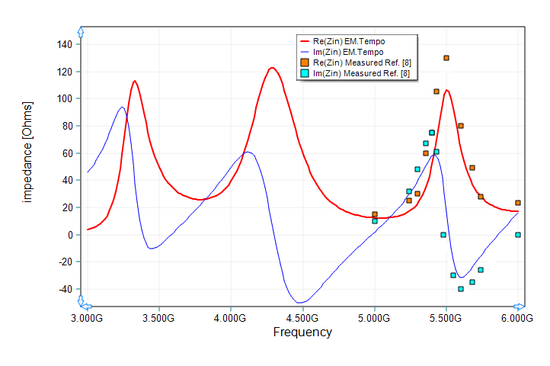Figure 29: Real and imaginary parts of the input impedance of the dielectric resonator antenna of Figure 26, solid red line: EM.Tempo results for input resistance, solid blue line: EM.Tempo results for input reactance, orange symbols: measured data given by Ref. [8] for input resistance, and turquoise symbols: measured data given by Ref. [8] for input reactance.

Figure 30: 3D far field radiation pattern of the spherical DRA with the coaxial feed computed at f = 4.5GHz by EM.Tempo.

Cylindrical DRA with an Edge Strip Feed

Next, we will examine a strip-fed cylindrical dielectric resonator antenna design as shown in Figure 31. The dielectric block has a radius of a = 10.3mm and a height of h = 34.3mm with a relative permittivity of ε_r = 9.4. A vertical metal strip of length L = 12mm and width w = 1mm is used to excite the cylindrical dielectric resonator in a similar manner to the rectangular DRA of Figure 2. One can use either the dielectric waveguide model (DWM) or tranverse resonance method (TRM) to derive the characteristic equation of the HEM_mnl modes of the cylindrical dielectric resonator. These equations involve a combination of the Bessel functions of the first kind J_n(x) and the modified Bessel functions of the second kind K_n(x). According to the analysis presented by Ref. [3], this particular cylindrical DRA shown in Figure 31 supports the HEM₁₁₁ and HEM₁₁₃ modes with resonant frequencies 2.90GHz and 3.72GHz, respectively. Figure 32 shows the FDTD mesh of the cylindrical DRA generated by EM.Tempo using a mesh density of 30 cells per wavelength along with high precision adaptive mesh settings.

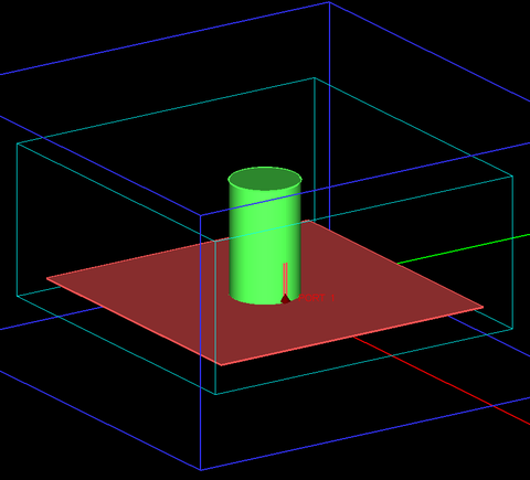Figure 31: Geometry of a cylindrical dielectric resonator antenna with a vertical metallic strip feed on its edge.

Figure 32: FDTD mesh of the cylindrical DRA with an edge strip feed.

This project was simulated using EM.Tempo, and the computed return loss of the DRA is plotted in Figure 33. This figure also shows the measured results presented by Ref. [3]. Similar to the previous cases, the dimensions of the metallic ground plane were not given in Ref. [3]. For this simulation, a PEC ground plane of dimensions 75mm × 75mm was used. Both EM.Tempo and Ref. [3] show a 10-dB bandwidth of 860MHz, but EM.Tempo's bandwidth is shifted up by 170MHz starting at 3.17GHz and ending at 4.03GHz.

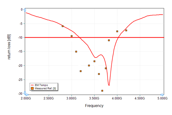Figure 33: Return loss of the cylindrical dielectric resonator antenna of Figure 31, solid red line: EM.Tempo (FDTD) results, red symbols: simulated data presented by Ref. [3], and blue symbols: measured data given by Ref. [3].

Figures 34 and 35 show the 3D far field radiation patterns of the cylindrical DRA at the two resonant frequencies f = 3.29GHz and f = 3.83GHz. From these two figures, the directivity of the DRA is seen to be 6.76dBi and 9.35dBi at f = 3.29GHz and f = 3.83GHz, respectively. Ref. [3] reports measured antenna gain values of 7dBi at 3.29GHz and 10dBi at 3.83GHz.

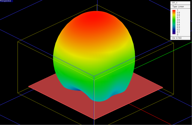Figure 34: 3D far field radiation pattern of the cylindrical dielectric resonator antenna of Figure 31 computed at f = 3.29GHz by EM.Tempo.

Figure 35: 3D far field radiation pattern of the cylindrical dielectric resonator antenna of Figure 31 computed at f = 3.83GHz by EM.Tempo.

Circularly Polarized Cylindrical DRA

Finally, we examine a circularly polarized (CP) cylindrical dielectric resonator antenna design presented by Ref. [3] and shown in Figure 36. The cylindrical dielectric resonator in this case is identical to the previous case: a = 10.3mm, h = 34.3mm, and ε_r = 9.4. Two identical vertical metal strips of length L = 11.5mm and width w = 1mm are used to excite the cylindrical dielectric resonator at two orthogonal polarizations, one located on the x-axis and the other on the y-axis. There is a thin substrate of thickness d = 0.762mm and relative permittivity ε_r = 2.93 underneath the metal ground plane. The two feeding vertical metal strips are connected to two horizontal microstrip lines of width w₀ = 1mm on the other side of the substrate by two vertical wire lines passing through two small holes in the ground plane as shown in Figure 37. The two feeding microstrip lines are connected to the outputs of a quadrature hybrid coupler shown in Figure 38. The input and isolation port lines have a width of w₁ = 1.94mm. The side dimension of the hybrid is L₁ = 14.67mm. The width of the arms parallel to the input port line is w₁ = 1.94mm and the width of the arm orthogonal to the input port line is w₂ = 3.21mm.

Figure 36: Geometry of a circularly polarized cylindrical dielectric resonator antenna fed by two vertical metallic strips on two orthogonal locations.

Figure 37: Connection of vertical metal strips to a hybrid coupler network on the opposite side of the underlying substrate through small holes in the ground plane.

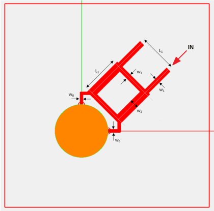Figure 38: Geometry and dimensions of the planar hybrid coupler.

This project was simulated using EM.Tempo, and the computed return loss of the DRA is plotted in Figure 39. This figure also shows the measured results presented by Ref. [3]. Similar to the previous case, the dimensions of the metallic ground plane were not given in Ref. [3]. A PEC ground plane of dimensions 80mm × 80mm was used for this FDTD simulation. EM.Tempo predicts a large -10dB bandwidth of 850MHz spanning from 3.08GHz to 3.93GHz.

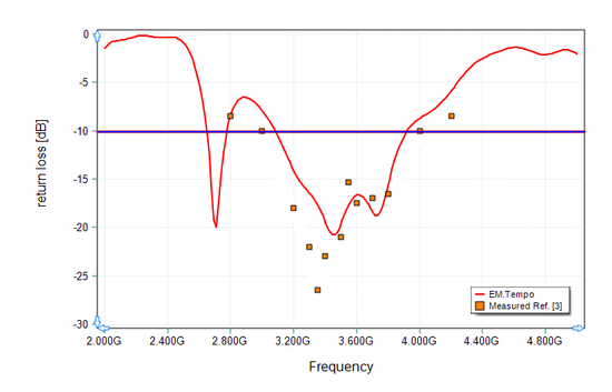Figure 39: Return loss of the CP cylindrical dielectric resonator antenna of Figure 36, solid line: EM.Tempo results, symbols: measured data given by Ref. [3].

Figure 40 shows the 3D far field radiation patterns of the CP cylindrical DRA at f = 3.3GHz. Figures 41, 42 and 43 show plots of the 2D polar radiation pattern of the CP antenna in the two principal YZ and ZX planes and an additional φ = 45° plane, respectively. Figure 44 shows the computed axial ratio of the cylindrical dielectric resonator as a function of the elevation angle θ expressed in radians in the three YZ, ZX and φ = 45° planes. A fairly good circular polarization performance is observed over a wide angular field of view.

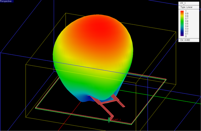Figure 40: 3D far-field radiation pattern of the cylindrical dielectric resonator antenna of Figure 36 computed at f = 3.3GHz by EM.Tempo.

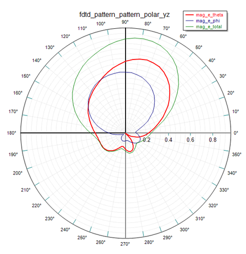Figure 41: 2D polar radiation pattern of the cylindrical dielectric resonator antenna of Figure 36 in the YZ principal plane.

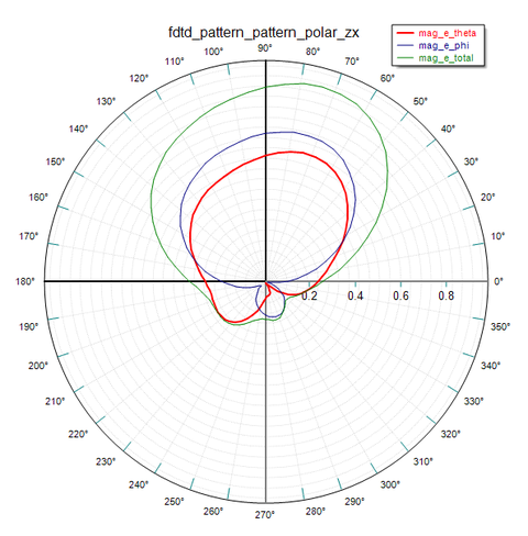Figure 42: 2D polar radiation pattern of the cylindrical dielectric resonator antenna of Figure 36 in the ZX principal plane.

Figure 43: 2D polar radiation pattern of the cylindrical dielectric resonator antenna of Figure 36 in the φ = 45° plane.

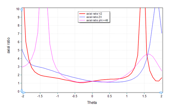Figure 44: Axial ratio (AR) of the cylindrical dielectric resonator antenna of Figure 36 as a function of the elevation angle in the YZ, ZX and φ = 45° planes.

In the above simulation, the isolation port line of the quadrature hybrid coupler was left open-ended. If we terminate this port in a matched 50Ω resistive load, the bandwidth of the DRA will increase. Figure 45 shows the terminated hybrid structure, where a short vertical line hosting a resistive lumped device is connected to the end of the isolation.

Figure 45: Terminating the isolation port line of the quadrature hybrid in matched load.

Figure 46 shows the computed return loss of the CP cylindrical DRA with a matched termination. EM.Tempo predicts an almost doubled -10dB bandwidth of 1630MHz spanning from 2.9GHz to 4.53GHz.

Figure 46: Return loss of the CP cylindrical dielectric resonator antenna of Figure 45.

References

[1] A. Elsherbeni and V. Demir, The Finite-Difference Time-Domain Method for Electromagnetics with MATLAB Simulations. Scitech Publishing Inc. Chapter 9, Section 4, pp. 307-310, 2009.

[2] B. Li and K.W. Leung, "Strip-fed rectangular dielectric resonator antennas with/without a parasitic patch", IEEE Trans. Antennas & Propagat., vol. 53, No. 7, pp. 2200-2207, 2005.

[3] K.W. Leung, "Developmentof dielectric resonator antenna (DRA)", presented to the IEEE LI Section of Antennas & Propagation Society, October 2012.

[4] A. Buerkle, K. Sarabandiand, and H. Mosallaei, "Compact slot and dielectric resonator antenna with dual-resonance, broadband characteristics", IEEE Trans. Antennas & Propagat., vol. 53, No. 3, pp. 1020-1027, 2005.

[5] K.W. Leung, "Conformal strip excitation of dielectric resonator antenna", IEEE Trans. Antennas & Propagat., vol. 48, No. 6, pp. 961-967, 2000.

[6] K.W. Leung, K-M Luk, K.Y.A. Lai, and D. Lin, "Theory and experiment of an aperture-coupled hemispherical dielectric resonator antenna", IEEE Trans. Antennas & Propagat, vol. 43, No. 11, pp. 1092-1098, 1995.

[7] K.W. Leung, "Analysis of aperture-coupled hemispherical dielectric resonator antenna with a perpendicular feed", IEEE Trans. Antennas & Propagat., vol. 48, No. 6, pp. 1005-1007, 2000.

[8] K.W. Leung, K.M. Luk, K.Y.A. Lai, and D. Lin, "Theory and experiment of a coaxial probe fed hemispherical dielectric resonator antenna", IEEE Trans. Antennas & Propagat., vol. 41, No. 10, pp. 1390-1398, 1993.

---

Back to the Top of the Page

Check out more Articles & Notes

Back to EM.Cube Main Page