NeoScan Manual Part B: Measurement Preparations

Measurement Preparations

Signal Strength Check

You should have a reasonably large enough EO signal in order to perform a measurement or scan. In other words, the EO signal level must be much higher than the noise level (-90 dBm) as shown in Figure 3.1. Therefore, you have to do a quick check to see if your signal strength is strong.

Figure 3.1: A typical EO signal in Spectrum Analyzer.

Requirements during the Signal Strength Check

The following instruments are needed for a signal strength check:

1. NeoScan optical mainframe

2. Either one normal or one tangential probe

3. One Coplanar Waveguide (CPW) board for generating electric field

4. A RF Lock-in amplifier

5. A signal generator

6. A synthesizer for generating RF source to device under test

7. A 2nd synthesizer for mixing Local Oscillator (LO) source

8. Probe fixture

9. One GPIB-USB cable for Lock-in amplifier (Figure 3.2)

   

   

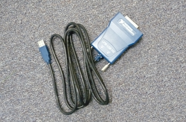   Figure 3.2: GPIB-USB cable.

10. One BNC – SMA cable

11. One USB multi-port Hub

12. One USB cable for optical mainframe

13. SMA RF cables

14. BNC cables for 10 MHz reference

Signal Strength Check Setup and Procedure

It is assumed that NeoScan optical mainframe is already on. Figure 3.3 shows the set up for a signal strength check.

Figure 3.3: NeoScan Signal Strength Test and Optimization.

1. Gently unwind the fiber and deploy the sensor head(s) at measurement location or on the probe fixture.

2. Gently clean and attach the appropriate fiber connector to the correct fiber port of the NeoScan system (Probe 1, Probe 2, or Probe 3).

   • Do not excessively pull or bend the fiber.

   • Do not bend or strike the probe tip.

3. Make sure all cables and fibers are in safe positions.

4. Secure the probe on probe fixture. If you are using a 2-axis translation stage, gently insert the probe inside the hole located on probe holder and fasten the screws – see sections 2.3 and 2.8 for more details.

5. Rotate the tangential probes around to align crystal E-field sensitivity direction to the field, see Figure 3.4.

   

   

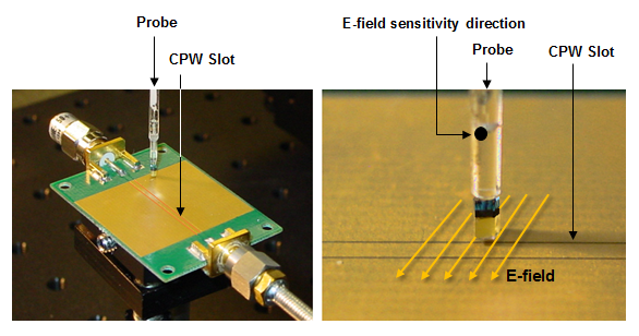   Figure 3.4: Positioning a probe above the slot of a Coplanar Waveguide (CPW).

6. Connect the U-jumper RMA cable from “Signal Out” to “RF In” in Channel 1, 2 or 3 as shown in Figure 3.5.

   

   

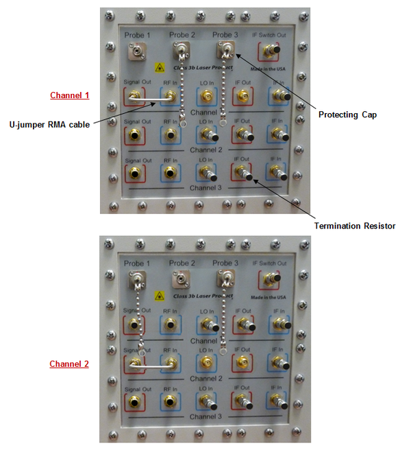   Figure 3.5: NeoScan Rear Pane set for Channel 1(top) and Channel 2 (bottom).

7. Set up the Signal Generator for Lock-in amplifier. Plugging its power cord into an electrical receptacle. Set it as 100 MHz and 0 dBm. Connect the signal generator output to Lock-in amplifier reference input (“REF IN”) on its front panel.

8. Set up Lock-in amplifier. Plugging its power cord into an electrical receptacle. Connect the GPIB-USB cable from the (back panel of) Lock-in amplifier to USB Hub (Figure 3.6).

   

   

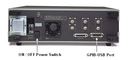   Figure 3.6: Rear panel of Stanford Research Systems SR844 RF Lock-In Amplifier.

9. Connect the “IF Out” on mainframe front panel to the “Signal In” on Lock-in amplifier using a BNC – SMA cable.

10. Set up a RF synthesized signal generator for generating RF source to the CPW. Plug its power cord into an electrical receptacle. Connect RF synthesized signal generator to CPW feed using a SMA cable. Set the operating frequency fo (GHz).

11. Set a 2nd RF synthesized signal generator for mixing Local Oscillator (LO) source. Connect it to “LO In” on the front panel of optical mainframe with a SMA cable. Set the frequency to fo + 0.1 (GHz) and the power to +15 dBm (regardless of the frequency). The NeoScan system will receive RF signals from the Electro-optic probe. The signal is then amplified and ultimately mixed with the output of the second RF synthesized signal generator. The mixed signal is then fed into the Lock-in amplifier, where the amplitude and phase are measured. For example, if your RF source to the CPW is set at 1 GHz, the correct setting for the 2nd synthesized signal generator would be either 0.9 GHz or 1.1 GHz. This provides a 100 MHz signal out of the IF Out port on the NeoScan optical mainframe with an amplitude equal to at the Signal Out/RF In connection. This is the signal being fed into the Lock-in amplifier Signal In port.

12. Connect the 10 MHz Reference OUT in the back panel of the signal generator (as the driving source for the 10 MHz synchronization network) to the 10 MHz Reference IN of the two RF synthesized signal generator using BNC cables. The Lock-in amplifier does not have a 10 MHz Reference input. The RF output of the 100 MHz signal generator (set to 0 dBm) is then connected to the Ref In on the Lock-in amplifier. This will synchronize the Lock-in amplifier to the synchronized synthesizers. Alternatively, you can select the 100 MHz signal generator to be the master and connect its 10 MHz Reference Out to the 10 MHz Reference In on the RF synthesized signal generator. Then connect the 10 MHz Reference out of the RF synthesized signal generator to the 10 MHz Reference In on the 2nd RF synthesized signal generator.

13. Turn the signal generator on. Make sure its “Modulation Generator” key is off.

14. Turn on Lock-in amplifier. The on/off power switch is located in the rear panel (Figure 3.6).

15. Turn the RF synthesized signal generators on. Toggle the front panel RF ON/OFF key to turn on RF power to the “RF OUTPUT” port. The display “RF ON” annunciator will turn on.

16. Bring the probe down close to the surface of CPW in such a way that the probe positions right above the CPW slot and move it around the slot to detect an EO signal.

    • To get the maximum EO signal, use a microscope (and a lamp for the microscope illumination) to adjust the probe height with the Z micrometer on the XY Linear Translation Stage.

17. Open NeoScan Optical Bench Manager program.

NeoScan Optical Bench Manager Program

NeoScan Optical Bench Manager program monitors optimization status of the system. The optimization process finds the polarization status of the polarization controller, and saves the optimized parameters and corresponding optical powers into the files.

Open NeoScan Optical Bench Manager program by double clicking on NeoScanOBM icon on desktop or Windows Explorer. The user interface of the program consists of two pages: System Monitor page and Optimization Settings page (Figure 3.7). By default, the program opens up with “System Monitor” page.

Keep NeoScan Optical Bench Manager program running until the end of the experiment or measurement.

Figure 3.7: NeoScan Optical Bench Manager Program.

System Monitor Page

When the program starts, the system detects the total return power and the polarization power in the channel, plots their variations over time and displays their numerical values in mW. Figure 3.8 indicates that channel 1 is selected to deliver the beam to optical probe with Probe ID No. 1505. The Probe ID No. is a four-digit integer number provided by EMAG Technologies Inc. The green “Probe Detected” indicator indicates that the probe is connected to the correct channel.

Figure 3.8: The total return power and the polarization power of delivered beam to the optical probe with Probe ID No. 1505 in channel 1.

1. Select the channel number you want to use for the measurement using the dropdown list labeled “Select Channel” (Figure 3.9). “Ch n” denotes channel n where n = 1, 2, ... NeoScan Optical Bench Manager program opens up with the “Ch 1” as the default working channel.

   

   

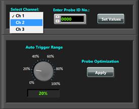   Figure 3.9: Selecting the working channel from NeoScan Optical Bench Manager window.

2. Enter “Probe ID No.” as the number marked on the fiber associated with the probe.

3. Press “Set Probe ID” button to update (Figure 3.8).

   • When either the total return power or the polarization power is too low (less than 0.3 mW), the information panel will remind a user to correct the problem. This can be the case if the probe is not connected or is defective.

   • When the user presses “Set Values” button, the previous (existing) saved optimization parameters/voltages will be applied to the polarization controllers of the selected channel. The program will check whether the polarization state is maintained or not.

4. To start a new probe optimization press “Apply” button.

If the polarization is maintained, the total return power and the polarization power will lie within the specified optimized range (the default value is ±20%). In this case, “Optimization Indicator LED” becomes green. Otherwise, it start blinking and the information panel indicates: “Polarization is not maintained: Optimization is required.” A user can change the threshold from the box labeled “Auto Trigger Margin” (see Figures 3.7 and 3.8). If the power difference is greater than 20%, the polarization state is found not to be maintained, therefore, the user will be prompted with a dialog window giving an opportunity to initiates the optimization process or skip the optimization by choosing “No.”  

The “Stop” button stops the application. To close (kill) the NeoScan window click on exit button on the top far right in the LabView user interface. To re-start running the program press the start button located on the top left in the LabView window as shown in Figure 3.10. During the run, the start button will disappear. Keep NeoScan Optical Bench Manager program running until the end of the measurement.

Figure 3.10: Start and Stop buttons for NeoScan Optical Bench Manager.

• The message box in “Information Panel” displays messages of warnings, actions and results.

• “Save Plots” saves in folder C:\ProgramData\NeoScan\OpticalBenchHistory.

• A user can reset the graphs by pressing “Reset Plots” button. The updated start time will be displayed under the power graph after “Started at” and in the information panel.

• There are two options to display power plots: The “Entire History” option displays the power plots from the time Optical Bench Manager program started (numerically is displayed as Start Project Time in information panel). The “Updated” option displays the power plots after resetting the plots (pressing “Reset Plots” button), see Figure 3.11.

  

  

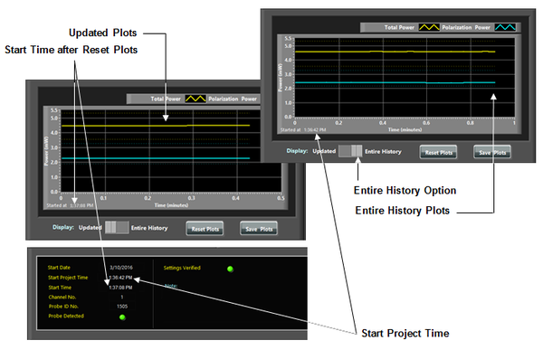  Figure 3.10: Resetting the power plots and displaying them with the Entire History and Updated options.

 

Optimization Settings Page

To set the optimization parameters, press “Optimization Settings” tab in NeoScan Optical Bench Manager program (Figure 3.11): Make sure the GPIB-USB cable from the back panel of Lock-in amplifier is connected to the NeoScan USB Hub.

Figure 3.11: Optimization Settings page in NeoScan Optical Bench Manager program.

1. Set Lock-in amplifier from “Lock-in Amplifier Settings” section (Figure 3.12). Put down the Visa menu and select the appropriate GPIB address for Lock-in amplifier Visa. The default is GPIB0::8::INST.

   

   

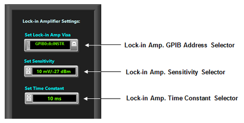   Figure 3.12: Lock-in Amplifier Settings in Optimization Settings Page.

2. If you change any value, press “Set Values” button to update.

3. Set Lock-in amplifier parameters:

   1. Set Lock-in amplifier sensitivity. The sensitivity of Lock-in amplifier is the rms amplitude of an input sine (at the reference frequency) which results in a full scale DC output (10Vdc).

   2. Select “Time Constant” from the dropdown lists. The default for time constant of the output low-pass filter that determines the bandwidth of Lock-in amplifier in 10 ms.

4. Press “Set Values” button to update.

Other parameters that should be directly set on SR844 RF Lock-in amplifier – since they are not controlled:

•  Time constant: 24 dB/oct, Figure 3.13(a).
•  Signal Input: 50  Low noise, Figure 3.13(b).
•  Sensitivity: Low noise, Figure 3.13(c).
•  X display: R(dBm), Figure 3.13(d).
•  Y display: θ, Figure 3.13(e).
•  Remote: 50 Ω external source, Figure 3.13(f).


Figure 3.13: Stanford Research Systems SR844 RF Lock-In Amplifier: (a) Time constant: 24 dB/oct, (b) Signal Input: 50 Ω Low noise, (c) Sensitivity: Low noise, (d) X display: R(dBm), e) Y display: θ, (f) Remote: 50 Ω external source.

The signal levels at the Signal In port on the Lock-in amplifier are in the range of -100 dBm to -40 dBm or higher, depending on device one measures. It is important to set the sensitivity of the Lock-in amplifier greater than the expected input signal amplitude at the Signal Input port (from the IF Out of the optical mainframe). For example, if you expect a signal less than -67 dBm but greater than -87 dBm, set the sensitivity to -67 dBm and 100 μV (rms) setting. If the input signal is greater than the input signal setting, an OVERLOAD condition will occur and the red LED OVERLOAD indicators on the Lock-in amplifier will flash.

• If the largest tolerable noise signal (at the input) exceeds the full scale signal, the red LED OVLD indicators in lock-in indicate that the readings may be invalid due to an overload condition. In this situation, you many try increasing the time constant or to use a larger full scale sensitivity.

5. Keep the default values for other parameters. Table 3.1 lists the default values for the main parameters used in the optimization process, see Figure 3.14.

6. Optimization parameters are stored in C:\ProgramData\NeoScan\OptimizationParameters folder.

Figure 3.14: Optimization parameters settings in Optimization Settings Page.

If the optical signal is low, check to make sure:

• The probe and the crystal on its tip is fine.

• The operating frequency is correct.

• All the components are connected correctly and appropriately.

• All instruments are functioning properly.

• All cables and the PM fiber are fine.

• All connectors are in good conditions – make sure they are not loose.

• CPW is functioning properly.

• Lower the probe down close to the surface of CPW and make sure the probe positions right above the CPW slot and move it around the slot.

Probe Optimization

The NeoScan software monitors and controls the polarization of the optical beam in the system. The optimization status for each probe at each channel needs be maintained for an extended period of time. Not only an initial optimization process for each probe at each channel is needed, but also additional optimization processes are needed if the status is not maintained. In general, you have to perform optimization whenever you detach the fiber connectors from the fiber ports of the NeoScan system or when the fluctuation in the total return optical power and the polarization power are varied more than 20%. After the optimization procedure, the system is ready for real-time measurement or scan.

Optimization Setup and Procedure

It is assumed that NeoScan optical mainframe is already on. The setup for the optimization procedure is similar to Signal Strength Check setup as described in section 3.1.2.

To get the maximum EO signal:

1. Move the probe around the CPW slot using the X or Y Miniature Translation Stages.

2. Position the probe right above the CPW slot.

3. Using the Z Miniature Translation Stage and lower the probe down close to the surface of CPW as much as possible.

NeoScan Optimization Utility Program

Figure 3.15: Dialog window for initiating the optimization process.

In order to initiate an optimization, it is assumed:

• The channel number and the Probe ID No. of the probe you want to optimize are selected.

• The steps described in section 3.2.2 in “Optimization Settings Page” have been done (GPIB address of the Lock-in Amplifier, Time Constant, and the Sensitivity, have been already chosen).

• Press “Apply” button to start new probe optimization (Figure 3.7).

A user is presented with a dialog window shown in Figure 3.15, giving an option to initiates the optimization process – which will take about 20 minutes to be completed – or skip the optimization by choosing “No.” Click on “Yes” for optimization. The system will remind a user to prepare an optimization structure. Align crystal field sensitivity direction to optimization structure field properly and press “Continue”.

When the optimization process starts, NeoScan Optimization Utility window will pop up, and the detailed optimization parameters are displayed to a user (Figure 3.16): Table 3.1 lists the main parameters used in optimization process with their default values. The change of the return power and the EO signal are plotted during the optimization process as shown in Figure 3.17, and their values are displayed in the boxes labeled “PD Power” and “EO Signal”, respectively. a user can monitor “Polarization Controller Parameters” through the information panel shown in Figure 3.18.

Figure 3.16: NeoScan Optimization Utility program.

Figure 3.17: Change of the return power and the electro-optic signal graphs during the optimization process (left to right direction indicates the start to the end of the process)

The optimization process takes about 20 minutes. It can be used to diagnose hardware failures. When the phase optimization has completed, the optimization window will prompt a user to perform a probe stability test through a red blinking “Start Stability Test” button at the bottom of the Window (Figure 3.19). To perform the probe fiber stability test, press the “Start Stability Test” button shown in Figure 3.19. An information dialog box will pop up and explains the procedure for the test. Press “Close” button in dialog box and then lift the middle of the fiber at least 2 m from either the probe head or the optical connector. Move it up and down, and/or left and right several times. The program will record variations in return power on the screen. Be sure not to pull the fiber at the connector or the probe ends. After performing this for approximately 30 seconds, press “End Stability Test” on the window. If signal fluctuations during the motion remains within the variation limit (default value is 1 dBm), the optimization is considered to be valid, otherwise, the program will repeat optimization (see Figure 3.20).

At the completion of the signal optimization process, the optimization window will disappear and the display will return to NeoScan Optical Bench Manager window. The optimized parameters will be written in files in ProgramData\NeoSca\OptimizationParameters.

You have to perform an optimization:

1. When you attach the fiber connectors to the fiber ports of the NeoScan front panel,

2. Whenever you detach a fiber connector from to the fiber ports of the NeoScan front panel and re-attach it to the same or the any other port.

3. When the fluctuation in the total return optical power or the polarization power are varied more than the defined threshold value (default value is 20%).

4. When there is an abrupt and sharp change in temperature.

• If the Probe ID No. is not correct, NeoScan Optical Bench Manager cannot find the files for optimization parameters, therefore, a user will be prompted with a warning dialog window shown in Figure 3.21.

When the voltages to the polarization controllers for a channel are set to the correct optimized values, you “may” observe a sharp change in the polarization power as shown in Figure 3.22. You can save the power plots by pressing “Save Figures” button.

Figure 3.18: Information Panel in NeoScan Optimization Utility program.

Figure 3.19: Stability Test in NeoScan Optimization Utility.

Figure 3.20: Comparison of a completed optimization process with a failed one in NeoScan Optimization Utility program.

Figure 3.21: Warning dialog window when the files for optimization parameters are not found.

Figure 3.22: The change in the polarization power after applying the optimization voltages to the polarization controllers.