Difference between revisions of "Analog Tutorial Lesson 2: Time and Frequency Domain Analysis of an RLC Filter"
Kazem Sabet (Talk | contribs) (→Running a Transient Test) |
Kazem Sabet (Talk | contribs) (→Running a Transient Test) |
||
| Line 108: | Line 108: | ||
Since the period of the input pulse waveform is 1ms, your specified time interval contains 5 periods. Both the source signal and output voltage signal are plotted on the same graph. The signal overshoot at the rise and fall of the pulse train are better visible here. In order to examine this transient behavior in more detail, change the transient test [[parameters]] as follows: | Since the period of the input pulse waveform is 1ms, your specified time interval contains 5 periods. Both the source signal and output voltage signal are plotted on the same graph. The signal overshoot at the rise and fall of the pulse train are better visible here. In order to examine this transient behavior in more detail, change the transient test [[parameters]] as follows: | ||
| − | |||
| − | |||
| − | |||
| − | |||
| − | |||
| − | |||
| − | |||
| − | |||
{| border="0" | {| border="0" | ||
Revision as of 20:42, 6 September 2015
Contents
What You Will Learn
In this tutorial, you will investigate a linear, time-varying, RLC circuit shown in the figure below. Using this circuit, you'll learn how to analyze transient and frequency domain responses.
Drawing the Circuit
We assume that at this point you have already completed Tutorial Lesson 1 and have acquired the basic circuit editing skills. If you haven’t, you may want to look over Tutorial Lesson 1 now. The following is a list of parts needed for this lesson:
| Part Name | Part Type | Part Value |
|---|---|---|
| V1 | Voltage Source | 1 |
| L1 | Inductor | 1u |
| C1 | Capacitor | 1n |
| R1 | Resistor | 50 |
Note that you can use the keyboard shortcuts L and C for placing inductors and capacitors in your circuit. 1n represents 1 nano-unit. It can also be entered as 1E-9, or 1NF. 1u is 1 micro-unit, which can also be entered as 1E-6. RF.Spice is case-insensitive, so you could enter 1 micro-unit as 1e-6, or 1E-6. Also, the type of the unit is ignored, so 1NF and 1ns are both equivalent to 1n. 1 n, however, will be interpreted as 1, since spaces are illegal in values. Place all the four parts listed above and connect them as shown in the figure using wires. For the time being, leave the voltage source as a default DC source with 1V voltage. Do not forget to define a ground for your circuit.
Setting Up and Running a Live Simulation
Recall that a "Live Simulation" is a continuous time domain simulation that runs indefinitely until it is paused or stopped and reset. Since simulations do not produce a graph, you will need to use Virtual Instruments to measure the circuit. Specifically, you will use a "Virtual Oscilloscope" in this lesson.
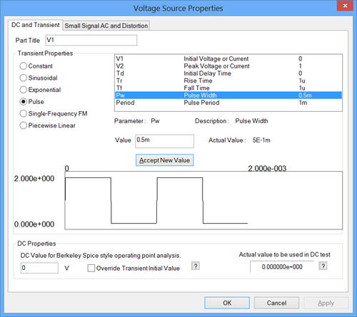
First, you are going to change the type of your voltage source V1 to a square wave generator. You may alternatively use the "Virtual Function Generator" for this purpose. Double-click the voltage source to open its property dialog. From the Transient Properties, select the "Pulse" option. The table on the right list the various properties of the Pulse Waveform. The default amplitude is 1V. Keep all the default values except for "Pulse Width" and "Pulse Period". Change their values to 0.5m and 1m, respectively. Note that these values represent milliseconds. A period of 1ms with a pulse width of 0.5ms corresponds to a pulse repetition rate (or frequency) of 1KHz, with a duty cycle of 50%. This is shown in the opposite figure.
Make sure circuit nodes are displayed. Your schematic should now look like the following figure:
Next, you will define the virtual oscilloscope. Go to the "Virtual Instrument Panel" on the right side of the screen and click on the button labeled "Add Meter". From the drop-down list, select "Oscilloscope". An empty oscilloscope window appears in the right side panel. Click the Setup button to expend the window and bring its settings dialog on. You should see a dialog like the figure below. Under the Traces tab, click the Input Trace 1 button to set up the first signal to measure on the oscilloscope. Set the input node to 1 and the reference node to 0. This will measure the voltage at node 1, which is where the voltage source is injected. Click on Input Trace 2 to set up the second signal. Set that input node to 2 and the reference to 0 and check the "Show" check box to display the signal. Workshop will try to automatically set the X and Y axis ranges to fit the signal into the graph window so you can leave all the other settings in the other tabs as they are.
Now click the "Run/Go" ![]() button of the Main Toolbar, or use the keyboard shortcut "Ctrl+G" to start the live simulation. Keep in mind that sometime B2.Spice may ask you to allow it to adjust certain simulation parameters like time step automatically. Click OK in such situations and let the program do its job. However, once the simulation starts, you may not see anything in the scope's display. Or there might be flashes of a signal, but no solid signals. When this happens, it is likely that Workshop is having trouble automatically setting one or both of the axis settings. Let's look at the axes settings to see what's happening.
button of the Main Toolbar, or use the keyboard shortcut "Ctrl+G" to start the live simulation. Keep in mind that sometime B2.Spice may ask you to allow it to adjust certain simulation parameters like time step automatically. Click OK in such situations and let the program do its job. However, once the simulation starts, you may not see anything in the scope's display. Or there might be flashes of a signal, but no solid signals. When this happens, it is likely that Workshop is having trouble automatically setting one or both of the axis settings. Let's look at the axes settings to see what's happening.
Switch on the Vertical tab. The Vertical V/Div is automatically set at 1. We know that the reading at node 1 should be the source signal set to 1V. Therefore, the 1V/div setting for the Vertical V/div should at least display the input signal correctly. Next, switch to the Timebase tab. The Timebase s/div setting is where the X axis range is set. It is set to "Auto" by default, but if you look closely, the setting might be continuously changing, probably due to the fact that one or both of the signals is throwing off the period calculations made by Workshop. In these cases, you can change the Timebase settings manually. To override this, click the "Manual" button. Let's set the signal to at least show the injected 1KHz signal. The period for our 1KHz pulse is 1ms. Since your graph has 10 divisions, the setting for time/div must be 1ms/10 = 0.1ms, or 100us. So enter 100u into the Timebase box and either press the Enter Key or click on the small "Return Arrow" button to accept the change. Otherwise, the dialog may show 100u, but Workshop will still be using the old value. Now you should see the signals in the scope's display screen.
If you look at the output waveform more closely, you will discern very small fluctuating signal overshoots at the rise or fall of the pulse. In the next part of this lesson, you will run a transient test to zoom in that portion of the temporal waveform.
Running a Transient Test
In the Toolbox on the left side panel, click on the "Tests" tab. Select the "Transient" option by checking the leftmost check box in the "basic" column. Then, click the "Setup" button in the Transient test row to open the test settings dialog as shown in the figure below. Set the Start Time to 0, Stop Time to 5m, Linearize Step to 1u and Step ceiling to 1u. Make sure that the Single Test tab is selected and the check box labeled "Graph" is checked in the "Output Results Options" section of the dialog.
Before running the test, you have to instruct B2.Spice what you want to plot at the end of the test. Click the button labeled "Preset Graph Plots...". A new dialog opens up, which looks like the figure shown above. Select the signals v(1) and v(2) and click the button labeled Add-> to move them to the graph table. Click the "Run Test" ![]() button of this dialog, or use the keyboard shortcut Ctrl+B to run the transient test. The following figure shows up at the bottom of the Workshop.
button of this dialog, or use the keyboard shortcut Ctrl+B to run the transient test. The following figure shows up at the bottom of the Workshop.
Since the period of the input pulse waveform is 1ms, your specified time interval contains 5 periods. Both the source signal and output voltage signal are plotted on the same graph. The signal overshoot at the rise and fall of the pulse train are better visible here. In order to examine this transient behavior in more detail, change the transient test parameters as follows:
| Start Time | 0 |
|---|---|
| Stop Time | 10u |
| Linearize Step | 1n |
| Step Ceiling | 1n |
Run the transient test once again and examine the new graph that replace the previous one. The transient behavior of the circuit in the first 10 microsecond is clearly visible now. You can further zoom in on that part of the graph. Make the graph view active and open the "Edit Axes" tab of the Toolbox.
Setting Up and Running an AC Sweep Test
The AC Sweep Test generates the frequency response of a circuit. When you run an AC sweep test, the voltage sources always act as sinusoidal signal sources regardless of the type you have specified in the property dialog of the individual sources. Furthermore, the frequency of that source signals will be stepped through a range of frequencies while the response of the circuit is recorded at each step.
Before you run an AC sweep test, you need to instruct B2.Spice which signal sources you want to treat as AC sources. To do so, double-click on your voltage source to open its property dialog. This dialog has two tabs. The first tab, which you saw earlier, is labeled as "DC & Transient". The second tab, which you should open now, is labeled as "Small-Signal AC & Distortion". At the top of the tab is a box labeled "Signal Offset" with units of V/A. When your circuit has active devices, it is important to set a DC bias point. This box will set the DC offset of your source. For this lesson, leave this box blank. Next, you will see a section titled "AC Properties for Small Signal AC Analysis Only". This section consists of boxes for Magnitude and Phase of the AC source plus the "Use Check Box". You have to check the last box to include the signal source in your AC analysis. Set the magnitude to 1V and phase to 0 degrees.
| |
You cannot run an AC sweep test if none of your signal sources has an AC designation. B2.Spice A/D will generate an error message. |
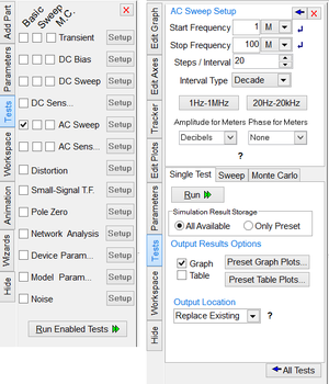
Next, open the Tests tab of the Toolbox, select the "AC Frequency Sweep" and click the Setup button to open the AC Sweep Settings Dialog. Enter 1MHz and 100MHz for the Start and Stop Frequencies, respectively, select the "Decade" option of "Step Interval", and set "Steps/Interval" to 20. These latter two specifications tell the simulator to step 20 points per each decade, and a decade is a factor of 10.
Before running the test, also specify the observables of your AC circuit simulation. Make sure that the Single Test tab is selected and the check box labeled "Graph" is checked in the "Output Results Options" section of the dialog. Click the button labeled "Preset Graph Plots...".
| |
An AC analysis involve complex-valued voltages and currents. You have to specify the format of the complex-valued signals. |
Select the signals vdb(1) and vdb(2) and click the button labeled "Add->" to move them to the graph table. This will produce plots of the magnitude of voltages at nodes 1 and 2 expressed in the dB scale. Click the "Run Test" ![]() button the test dialog, or use the keyboard shortcut "Ctrl+B" to run the AC sweep test. The following figure shows up at the bottom of the Workshop in a new Graph window:
button the test dialog, or use the keyboard shortcut "Ctrl+B" to run the AC sweep test. The following figure shows up at the bottom of the Workshop in a new Graph window:
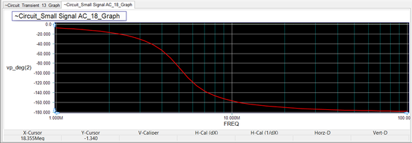
You will notice that the graph is in the form of a Bode plot. That is, the magnitude is plotted in decibels, 20*log(Y value), and the frequency is plotted on a log scale. Next, you will plot the phase of the signals. Remember that you set the phase of the AC voltage source to 0 degrees. Open the Edit Plots List Dialog once again. Select the two dB-magnitude graphs in the table on the right by highlighting them (use the Shift or Ctrl keys for multiple selection) and move them back to the signal table using the "<-Remove" button. Then, select the vp_deg(2) signal instead and move it to the graph table. Note that you will not plot the zero phase of the voltage at node 1. Run the AC sweep test once again and see the phase plot as shown in the figure below:


