NeoScan Manual Part D: Far Field Pattern Measurement
Contents
Far Field Patterns
Far Field Patterns

DXP = DXa+2 h tanθmaxX,
DYP = DYa+2 h tanθmaxY,
As the distance between the probe and the DUT surface increases, field components show broadened distribution and some details observed at shorter distance are no longer recognizable in the near field maps. However, near fields from a DUT at different probe heights (say 1 mm and 4 mm) generate relatively similar far field patterns.
Estimating the Optimal Antenna Scan Parameters
The “Height Settings” page in NeoScan Mapping Utility program estimates the optimal antenna scan parameters for far field pattern measurements. For instance, in order to calculate the far field patterns of a 34 mm x 34 mm 2.349 GHz patch antenna from a high resolution measured near field data, it is required that the probe height to be set at 1 mm with scan step size of 0.5 mm (500 μm). To achieve this you have to scan a total of 4624 points (68 x 68). However, the optimal antenna calculation suggests that you can achieve similar results for far field pattern by setting the probe 4 mm above the patch antenna and setting the step size at 1.995 mm. That is, you have to only scan 32 x 32 = 1024 points. This will deteriorate the near field resolution, yet it cuts the scanning time by half.
To measure the far field patterns you have to follow the procedure explained in section 4.2. However, before setting the scan parameters (discussed in section 4.2.4) in order to estimate the optimal values for the far field measurements parameters:
-
Press “Height Settings” tab in NeoScan Mapping Utility page (Figure 6.2).

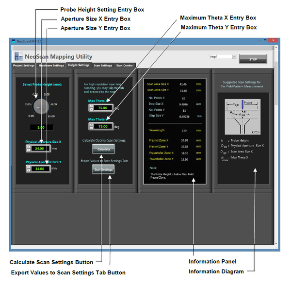 Figure 6.2: Aperture Settings tab in NeoScan Mapping Utility program.
-
Enter the DUT physical dimensions (in mm) in “Physical Aperture Size X” and “Physical Aperture Size Y” boxes (Figure. 6.3).
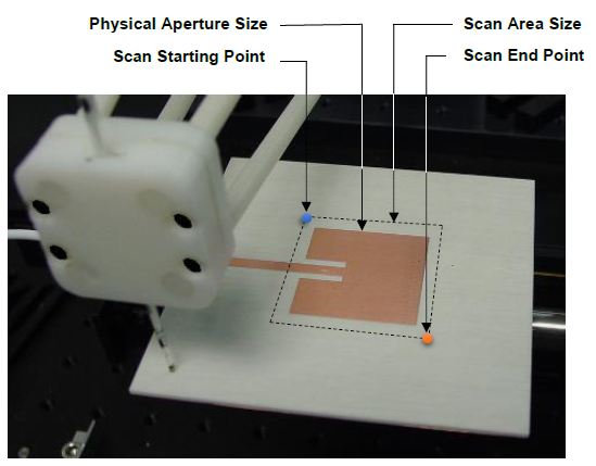 Figure 6.3: The scan starting and end points of a patch antenna.
 -
Choose the angular range (θmaxX, θmaxY) in degrees, over which the far field pattern calculation would be very accurate, in boxes named “Max Theta X” and ” Max Theta Y”.
-
Enter the “Probe Height.”
- By default, the “Probe Height” will be automatically set to λ/3. You can change this value by entering the new value in the box. “Wavelength” in information panel calculates the wavelength (λ) corresponding to the operating frequency.
-
Press “Calculate” button.
-
The program calculates the optimal scan area size, i.e., the starting point and the end point in a scan. For instance, the program suggests that the “Scan Area Size X” and “Scan Area Size Y” for a 34 mm × 34 mm 2.349 GHz patch antenna with a probe 1 mm about the antenna is 41.5 mm (Figures 6.3 and 6.4). That is, the scan starting point should be ½ (41.5 - 34) = 3.75 mm away from a corner of the antenna. “No. Points X” and “No. Points Y” in information panel present the suggested values for number of scanning points in X and Y directions and those of step sizes (in mm) will be displayed in “Step Size X” and “Step Size Y,” respectively.
-
Press “Scan Settings” button to export automatically the suggested values to the scan settings in “Scan Settings” page. Otherwise, the initial values in “Scan Settings” page are kept unchanged.
- The program returns the limits for the Fresnel and Fraunhofer Zones and give a notice whenever the probe height falls outside these zones (Figure 6.4). The Fresnel Zone is defined as 0.62√(𝐷3/𝜆), and the Fraunhofer Zones is expressed as 2𝐷2/𝜆 where D is DUT physical dimensions and 𝜆 denotes the operating frequency wavelength.
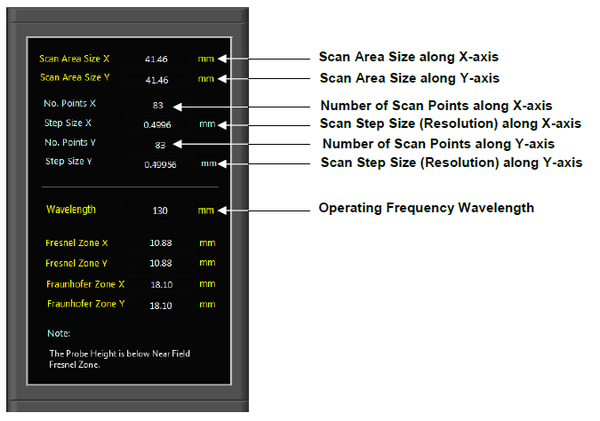 Figure 6.4: Information Panel for Aperture Settings Page.


Far Field Scans
NeoScan Visualization Utility program uses the near field maps of an antenna measured by the NeoScan system to estimate its radiation patterns using a near-to-far-field transformation based on the EM.Cube's FDTD simulation engine for far field calculations at the completion of an FDTD time marching loop. The main difference is that the FDTD Module uses a closed surface, known as the Huygens box, which completely encircles the radiating structure. In this case, however, NeoScan uses a 2D horizontal plane placed slightly above the surface of the antenna aperture. This plane, supposedly, must extend to infinity in the lateral directions. NeoScan Visualization Utility plots far field radiation pattern in both Cartesian and polar coordinate systems.
There are 13 parameters for far field calculation:
-
Press “Open File 1” button.
-
Choose the desired data file that will be used as Ex data file in Far Field Calculation and then press “OK” button in the dialog window (Figure 6.5).
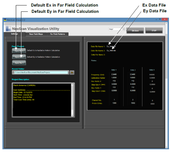 Figure 6.5: Selecting Ex and Ey data files for Far Field Patterns Calculation.
 -
Press “Open File 2” button.
-
Choose the desired data file that will be used as Ey data file in Far Field Calculation and then press “OK” button.
-
Press “Far Field Patterns” tab in NeoScan Visualization Utility program (Figure 6.6).
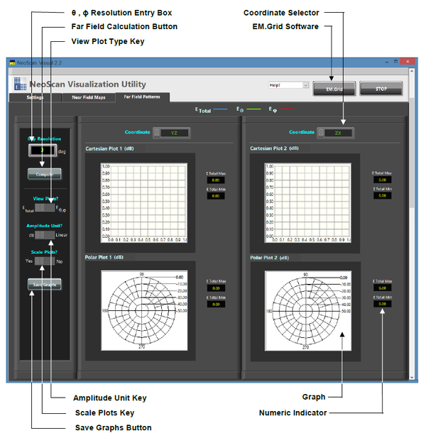 Figure 6.6: Far Field Patterns page in NeoScan Visualization Utility program.
 -
Set the resolution of calculation for θ and ϕ (in degree) from the box labeled “θ, ϕ Resolution.” The default value is 3°. Figure 6.7 presents the comparison of the far field radiation patterns for a 10.65GHz slotted waveguide with 1° and 5° resolutions.
- For this version of the software, Column corresponds to scan along +X (left to right), and Row corresponds to scan along +Y. Normal Direction of a DUT is considered to be along +Z. </li
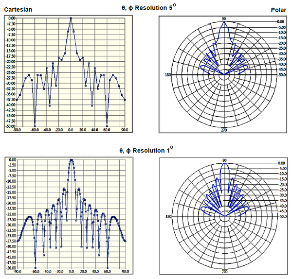 Figure 6.7: A comparison of the far field radiation patterns for a 10.65GHz slotted waveguide with 1° and 5° resolutions.
 -
Press “Calculation” button to call the far field executable engine to run.
- A black RUN window appears while the engine is running. It disappears as soon as the calculation is completed.
-
The output files for project “patch_2.349GHz” comprises the Cartesian Radiation Patterns in the XY, YZ, and ZX plane
- patch_2.349GHz_FF_PATTERN_Cart_XY.DAT
- patch_2.349GHz _FF_PATTERN_Cart_YZ.DAT
- patch_2.349GHz _FF_PATTERN_Cart_ZX.DAT
and the polar Radiation Patterns in the XY, YZ, and ZX plane
- patch_2.349GHz _FF_PATTERN_Polar_XY.ANG
- patch_2.349GHz _FF_PATTERN_Polar_YZ.ANG
- patch_2.349GHz _FF_PATTERN_Polar_ZX.ANG
They are written in C:\Users\neoscan\Documents\NeoScan\Projects\ patch_2.349GHz folder.
-
The radiation pattern is plotted in both Cartesian and polar coordinate systems (Figure 6.8). Use the “Coordinate” buttons to change the plane cut of the far field patterns to XY, YZ, or ZX.
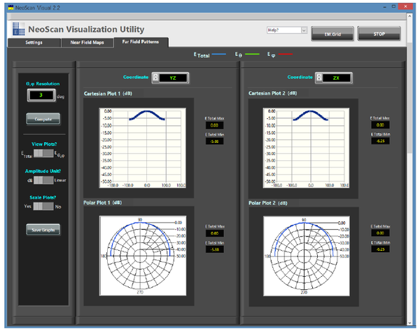 Figure 6.8: Cartesian and Polar plots of ETotal in dB for a path antenna.
 -
Switch a log scale graph to the linear one from the “Amplitude Unit” key.
-
A user has options to plot the total field (ETotal) or the θ and ϕ components (Eθ, Eϕ) of the field using the button labeled “View Plots?” (Figure 6.9).
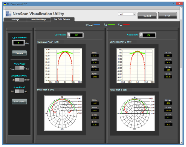 Figure 6.9: Cartesian and Polar plots of Eθ and Eϕ for a path antenna in linear scale.
 -
To compare plots use “Scale Plots?” button.
-
Use ‘Save Graphs’ Button to save all 12 pictures. The plots are saved in “Plots” folder in corresponding project folder.
-
EM.Grid is a Data Visualization and Calculation tool based on EM.Cube simulation environment, which provides the user with much more options for plotting the far field radiation as shown in Figure 6.10.
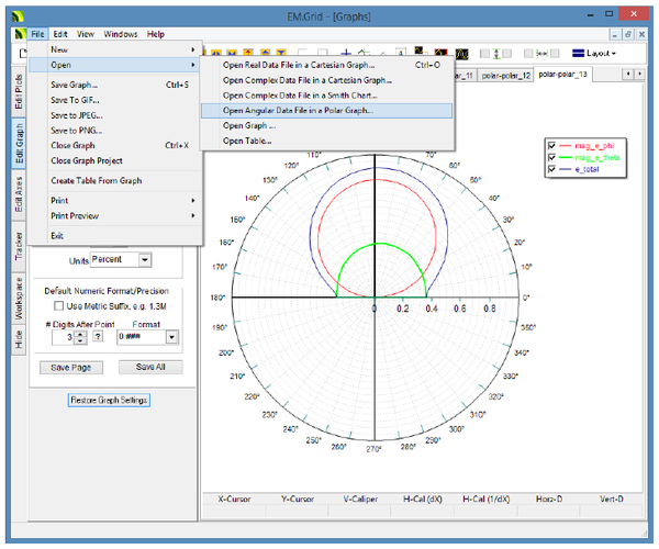 Figure 6.10: EM.Grid Data Visualization and Calculation Tools in NeoScan Visualization Utility program.


The “Stop” button stops the application. To close (kill) the NeoScan window click on exit button ![]() on the top far right in the LabView user interface. To re-start running the program press the start button
on the top far right in the LabView user interface. To re-start running the program press the start button ![]() located on the top left in the LabView window, see Figure 5.1.
located on the top left in the LabView window, see Figure 5.1.