EM.Tempo Tutorial Lesson 13: Analyzing the Radar Cross Section of the NASA Almond Target
Contents
Objective:
To import various target geometries to EM.Cube, excite them using plane wave sources and analyze their RCS using EM.Cube's FDTD simulator.
What You Will Learn:
In this tutorial you will import two STEP CAD models with complex geometries to EM.Cube. You will learn how to slice objects and set up slice planes. You will also define custom outputs based on EM.Cube's existing standard output quantities.
Getting Started
Open the EM.Cube application and switch to FDTD Module. Start a new project with the following attributes:
For this tutorial lesson, you need to download a STEP CAD files called "Almond_NSA.STP" from our File Repository.
Setting up the NASA Almond Structure
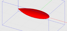
Import the CAD model "Almond_NSA.STP" to CubeCAD. You will see a collection of 150 black objects as the original color of their group is black. You can change the group's color in CubeCAD to make the objects more visible or leave them black as you will next move them to the FDTD Module.
Create a new PEC group called PEC_1 in the FDTD Module. Go back to CubeCAD, select all the 150 surface objects from the Navigation Tree and move them to the PEC_1 group in the FDTD Module. Define a plane wave source with the default TMz polarization, an incident Theta angle of 90° and an incident Phi angle of 0°.
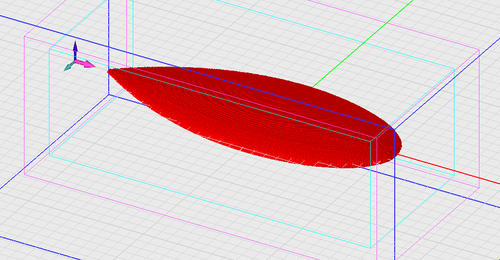
Generate and view the FDTD mesh using the default mesh settings. You will find a fairly coarse mesh of your almond-shaped target as shown in the figure below. Open the Mesh Settings Dialog and click the button labeled High Precision Mesh Settings at the top of this dialog. Pay attention to the values of minimum mesh density, minimum grid spacing for geometric contours and the absolute minimum grid spacing as a fraction of the average grid spacing in the free space. Click the Apply button of the dialog and see the new fine mesh generated. The new settings create a total of 6,312,570 cells.
Open the property dialog of the plane wave source and replace the value of the incident Phi angle with the variable "Phi". In this tutorial lesson, you are interested in the "Monostatic RCS" of the NASA almond in the azimuth direction. Define an RCS far field observable with the angle increment set to 3° for both Theta and Phi angles.
| |
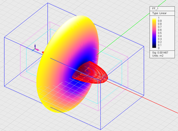
By default, EM.Cube computes the "Bistatic RCS", whereby the plane wave source is illuminated from a fixed direction and the RCS is calculated at all observation angles. EM.Cube can also alternatively compute the "Monostatic RCS" as a built-in sweep. In the latter case, the incident angles of the plane wave source are swept over the entire 3D space and the back-scattered RCS is computed and saved at RCS data files. The monostatic RCS results are shown as 3D visualization plots. |
Running the "Monostatic RCS" mode of the FDTD simulator can be computationally very intensive and time-consuming. There is a simpler way of doing the same since you are only interested in the azimuth RCS data. At the end of an FDTD simulation with a plane wave source and an RCS observable, a number of data files are generated. First, there is the often very large "FF_1.RCS" file that contains all the 3D RCS data for all the θ and φ observation angles. In addition, three more data files are generated: "FRCS.DAT", "BRCS.DAT" and "MRCS.DAT", recording the forward-scattered RCS, back-scattered RCS and maximum RCS values, respectively, in linear scale. When you run an FDTD analysis, these files contain a single value. When you run a sweep simulation, the data files contain sets of values corresponding to the sweep variable samples.
Defining a Custom Output
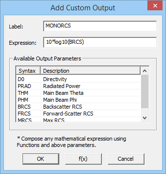
Before running a parametric sweep of your "Phi" variable, let's also define a custom output for your simulation. As mentioned earlier, the "BRCS.DAT" data file contains the monostatic RCS data in linear scale. Oftentimes, you see monostatic RCS plots expressed in dBm2 as a function of the angle in the literature. To verify your simulation results, you can define a new custom output that expresses the back-scattered RCS in dB scale. To do so, click the Custom Output button of the Simulate Toolbar or use the keyboard shortcut Ctrl+K to open the Custom Output Dialog. The dialog is initially empty. Click the Add button of the dialog to open the Add/Edit Custom Output dialog. Call the new output "MONORCS" and enter "10*log10(BRCS)" in the "Expression" box. At the bottom of the dialog, you can see a list of all the standard output quantities that EM.Cube generates for the given combination of sources and observables.
Close the "Add/Edit" Custom Output dialog. You will see that the name of your new custom output quantity, MONORCS, has been added to the list along with its definition. If you run an FDTD analysis, a new data file called "MONORCS.DAT" will be generated and listed in the Data Manager. If you run a parametric sweep, a data file called "MONORCS_Sweep.DAT" will be generated that contains the computed values of MONORCS for each sample of the sweep variable.
Running a Parametric Angular Sweep of the NASA Almond
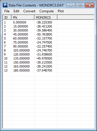
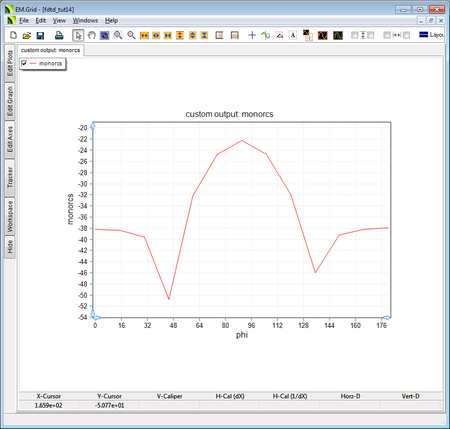
Run a parametric sweep of the almond-shaped target with "Phi" selected as the sweep variable. Set the start and stop values of Phi to 0° and 180°, respectively, and set the step value to 15°. Keep in mind that the polarization of your plane wave source is the default TMz, and the incident Theta angle has been fixed at 90°. At the end of the sweep simulation, open the Data Manager and plot the data file "MONORCS_Sweep.DAT" in EM.Grid. This is a graph of the monostatic (back-scattered) RCS as a function of the azimuth angle as shown in the figure below.
| |
This simulation may take a very long time, possibly several hours. If you have a multicore processor, use the single precision FDTD engine with as many thread as you have in your processor. |
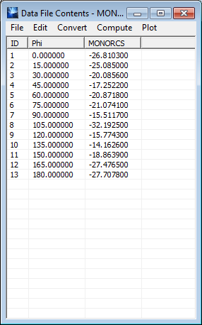
Next, change the polarization of the plane wave source to TEz and run the same parametric sweep of the "Phi" variable. The figure below shows the results for the TEz polarization.
